U2.5 實作：從 reference path 到 Flow ODE

本篇重用1 篇

• M2.3導航每 30 秒更新一次：Euler 法與它的誤差

設定：先固定其餘條件

沿用 U1.5 的 two-moons toy、MLP 與 random seed，只改 reference path、training target 與 sampler。這樣最後看到的差異才不會混入網路大小或資料不同。

本單元的符號是：

$$x_0=\text{起點 noise},\qquad x_1=\text{資料},\qquad t:0\to1.$$

它和 U1 的 diffusion 時間方向相反，寫程式前先把兩端對一次。

下載 Week 4：Flow Matching 與 ODE 取樣 notebook（.ipynb）

步驟一：製造 reference path

使用 Lipman 等人的 linear Conditional Flow Matching [1]，也就是 U2.1 的直線：

從端點製造 model input 與 label

$$\begin{gathered} \reveal{2}{x_t=(1-t)\reveal{1}{x_0}+t\reveal{1}{x_1},}\\ \reveal{3}{\dot I_t=x_1-x_0.} \end{gathered}$$

1. 1 抽出起點 noise $x_0$ 與資料 $x_1$。這一組配對同時決定中間的 input 與它的 label。
2. 2 抽出 $t$ 後，用直線插值得到 $x_t$。網路只會看到 $(x_t,t)$。
3. 3 對這條 reference path 微分，得到 $\dot I_t=x_1-x_0$。程式裡比較的就是 model output 與這個已知速度，再把 batch 的平方誤差取平均。

Training loop 只剩幾行：

for step in range(n_steps):
    x0 = torch.randn(batch, 2)       # 起點
    x1 = sample_data(batch)          # 終點
    t  = torch.rand(batch, 1)
    xt = (1 - t) * x0 + t * x1
    loss = ((model(xt, t) - (x1 - x0)) ** 2).mean()
    loss.backward(); opt.step(); opt.zero_grad()

網路看到的是 $(x_t,t)$，label 則是這一組端點的 reference velocity。它不需要知道 density，也沒有先算 posterior weights；L2 regression 會自己完成平均。

你應該會看到 loss 停在大於零的數字。U2.2 已經說明原因：同一個 $(x_t,t)$ 可能對應許多不同的 reference velocities，CFM loss 比理想 FM loss 多出的正是 conditional variance。Loss 不到零，不等於模型沒有學到 optimal velocity。

步驟二：沿著學到的 velocity 走

Euler sampler 是

@torch.no_grad()
def euler_sample(model, x0, n_steps):
    x, h = x0, 1.0 / n_steps
    trajectory = [x]
    for i in range(n_steps):
        t = torch.full((x.shape[0], 1), i * h, device=x.device)
        x = x + h * model(x, t)
        trajectory.append(x)
    return torch.stack(trajectory)

先固定一批 $x_0$，分別用 10、50、1000 步生成。檢查兩件事：

1. 步數增加後，終點 distribution 是否逐漸穩定；
2. 圖上的 trajectories 是否等於 training 時畫的直線。

第二題的答案通常是否定的。Training 的直線可以交叉；生成時的 ODE trajectories 跟著 posterior-average velocity，必須繞開那些交叉點。

步驟三：量出 velocity 變化的代價

U3.0 的直覺是：隔很久才重新確認時，方向或速度大小改得越多，越容易走錯。現在固定 exact velocity，把模型誤差拿掉，只比較 solver 與 trajectory。

在 log-log 圖上：

• 斜率主要反映 solver order：Euler 約為 $-1$，Karras 等人 [2] 在 diffusion sampling 採用的 Heun method 約為 $-2$；
• 同一斜率下的高度反映 trajectory 的 error scale；沿途 velocity 變化越大的 path，通常需要更多步。

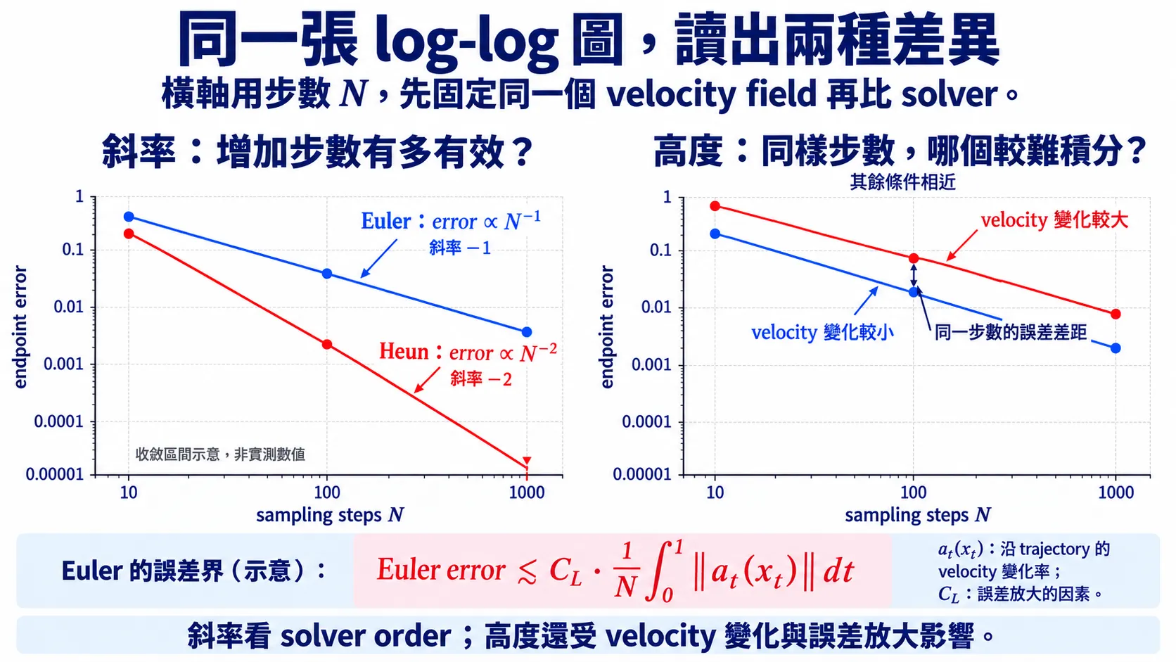
圖：log-log 圖的斜率與高度。 橫軸是步數 $N$，不是步長 $h$；在 $h=1/N$ 的收斂區間中，Euler 與 Heun 的斜率分別約為 $-1$、$-2$。右圖固定 solver，誤差高度除了沿 trajectory 的 velocity 變化，也受誤差放大因素影響；更精確的界會在 U3.1 推出。曲線為示意，非實測結果。

量測提醒先把分岔錯誤與離散化誤差分開

少數粒子可能因為步數不同而走向不同 mode。這種誤差是 $O(1)$，不會隨步長平滑下降，混進平均後會蓋掉 solver order。

因此 notebook 同時畫 median 與 mean：median 用來讀離散化收斂，mean 則保留「走錯 mode」這個真實但不同的問題。

步驟四：把 U1 的 denoiser 換成 velocity

載入 U1 在 VP path 上訓練的 $\epsilon_\theta$。依照 U2.3：

def eps_to_velocity(eps_model, x, t):
    a, s = vp_alpha(t), vp_sigma(t)
    da, ds = vp_alpha_dot(t), vp_sigma_dot(t)
    eps = eps_model(x, to_ddpm_time(t))
    return (da / a) * x + (ds - da * s / a) * eps

用 ODE sampler 積分這個 velocity，再與 deterministic DDIM 比較。時間格越細，兩邊的 trajectories 與終點應越接近；剩下的差異來自離散方式與時間格點，而不是另一個模型。

不能。eps_to_velocity 裡的 $(a,s,\dot a,\dot s)$ 必須來自模型 training 時看過的 path。換輸出座標不需要重訓，換中間 distribution 則需要。

作業

1. 非 Gaussian 起點。 把 $x_0$ 換成 $[-2,2]^2$ 的 uniform distribution，重新訓練並畫出 trajectories。哪些程式碼不必改？
2. Coupling。 保持 $p_0$、$p_1$ 不變，比較 independent pairing 與 minibatch 內依位置配對。畫出 reference paths、ODE trajectories 與少步誤差。
3. Path。 固定 pairing，只把 linear path 換成 time-reversed VP path。比較兩者的 marginal trajectories；不要用 conditional paths 的形狀直接猜答案。
4. Solver。 對同一個 velocity field 比較 Euler 與 Heun，從 log-log 圖估計斜率。

快速回顧一下

想一想

Linear CFM 的 training loss 停在大於零，最可能的原因是什麼？ ODE 無法生成資料。 同一個 $(x,t)$ 可能有多種 reference velocities，CFM loss 包含不依賴模型的 conditional variance。 直線不能微分。

看解答

想一想

把 VP denoiser 轉成 velocity 後，哪一項仍然不能在不重訓下更換？ ODE solver。 Noise／velocity parametrization。 模型 training 時使用的 probability path。

看解答

參考文獻

1. Lipman, Y., et al. Flow Matching for Generative Modeling. ICLR 2023.
2. Karras, T., Aittala, M., Aila, T., Laine, S. Elucidating the Design Space of Diffusion-Based Generative Models. NeurIPS 2022.