M1.1 Guessing Height from Shoes: Conditional Expectation

Only the shoes are visible

A photograph shows shoes of size 25 cm, and you must guess the wearer’s height.

What value would you predict, and why?

How would additional group information change your prediction?

A natural rule averages heights among people with the same observed features. We use illustrative groups and numbers, not an empirical demographic model. How are coarse and fine group averages related?

DiscussionQ1

What generates the random variables, what average is predicted, and what changes when we learn another feature?

Show the reasoning

Identify the source of randomness as well as the measured height.

A person is randomly drawn from a population, producing jointly distributed height $Y$ , shoe size $X$ , and group label $G$ .

Given $X=25$ , average heights under that conditional population. This is a group center, not a guaranteed individual height.

Additional $G$ divides the same shoe-size group into finer groups. Their weighted averages must recombine into the original average.

Group, average, and recombine

A table maps each shoe size to its group’s average height. Observing size selects the corresponding table entry.

Refining groups does not replace the population. Weighting fine-group means by their conditional proportions recovers the coarse mean. Individual fine groups can still have larger variance.

Additional information can move a prediction up or down; those changes average back to the original prediction.

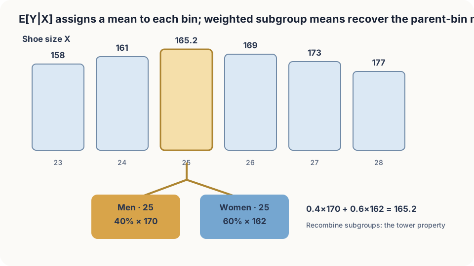
Fine conditional groups recombine into their coarse group using population proportions.

Figure: conditional expectation labels each group with its mean; the tower property recombines the labels.

Define the group average

For jointly distributed $X,Y$ , define

m(x)=\mathbb E[Y\mid X=x] =\sum_y yP(Y=y\mid X=x), \quad\text{or}\quad\int y\,p(y\mid x)\,dy.

For fixed $x$ this is a number. Substituting random $X$ gives $m(X)=\mathbb E[Y\mid X]$ , itself a random variable determined by the observed information. In continuous settings, use a suitable version of the regular conditional law where defined.

Useful properties.

Total expectation: averaging all group means gives $\mathbb E[Y]$ .
Tower property: refining and then averaging back gives

\mathbb E\big[\,\mathbb E[Y\mid X,G]\;\big|\;X\,\big]=\mathbb E[Y\mid X].

The fine $(X,G)$ average returns to the coarse $X$ average. 3. Take out known factors: $\mathbb E[h(X)Y\mid X]=h(X)\mathbb E[Y\mid X]$ under integrability. 4. Independence: if $X$ and $Y$ are independent, every conditional mean equals the overall mean.

DetailsProve the discrete tower property

Fix $X=x$ , then weight the finer conditional means by $P(G=g\mid X=x)$ :

\sum_g P(g\mid x)\sum_y y\,P(y\mid x,g)=\sum_y y\sum_g P(y,g\mid x)=\sum_y y\,P(y\mid x)=\mathbb E[Y\mid X=x].

Use conditional-probability multiplication and sum out $g$ . The continuous proof replaces sums by integrals under the appropriate integrability assumptions.

Two guesses and one consistency relation

The first guess reads the shoe-size group’s center. The next note explains why squared error favors that center rather than another statistic.

The refined guesses must average back: for illustrative means 170 and 162 with proportions 0.4 and 0.6, the coarse mean is 165.2. Two positively weighted subgroup means cannot both exceed their combined mean.

What does extra information improve? With finite second moments, total variance gives

\mathrm{Var}(Y\mid X) =\mathbb E[\mathrm{Var}(Y\mid X,G)\mid X] +\mathrm{Var}(\mathbb E[Y\mid X,G]\mid X).

The expected remaining within-group variance cannot increase. This does not require every individual fine group’s variance to be smaller.

These are population identities. A different source population may require a different table. Estimating the table from limited data also becomes unstable when grouping leaves too few examples per cell.

Simulate a synthetic population

import numpy as np
rng = np.random.default_rng(1)
def population(n):
    g = rng.random(n) < 0.5
    shoe = np.where(g, rng.normal(26.5, 1.0, n), rng.normal(23.5, 1.0, n))
    height = np.where(g, 176 + 4*(shoe-26.5), 158 + 4*(shoe-23.5)) + rng.normal(0, 5, n)
    return g, shoe, height
for n in (200_000, 60):
    g, shoe, h = population(n)
    b = np.abs(shoe - 25) < 0.25
    pm = g[b].mean()
    EY, EYm, EYf = h[b].mean(), h[b & g].mean(), h[b & ~g].mean()
    print(n, b.sum(), EY, EYm, EYf, pm*EYm+(1-pm)*EYf)

When both empirical subgroups are nonempty, their size-weighted means reproduce the empirical coarse mean exactly. With only 60 observations, narrow subgroups can be nearly empty or empty, exposing estimation instability and undefined sample averages.

Check your understanding

References

Grimmett, G., Stirzaker, D. Probability and Random Processes, 3rd ed. Oxford University Press 2001.
Williams, D. Probability with Martingales. Cambridge University Press 1991, Ch. 9.
Blitzstein, J. K., Hwang, J. Introduction to Probability, 2nd ed. CRC Press 2019, Ch. 9.