L4.5 Where should instructions enter a shared model?

Builds on2 notes

• M0.2Thirty Seconds Without GPS: Taylor Expansion and Straight-Line Prediction
• M1.1Guessing Height from Shoes: Conditional Expectation

One machine, different instructions

The same photograph can be brightened or turned into a night scene. The photograph alone does not specify which answer is wanted. Where does the instruction enter the network? Write this extra information as a condition $c$:

• “Make this a night scene”: a category condition.
• “Generate from this description”: a sequence of tokens.
• “We are at step 300; perform the appropriate correction”: a scalar condition.

The last condition describes the algorithm’s state, rather than a user instruction. Shared weights perform different operations at different stages, so the stage must be supplied.

Conditions can enter the input, modulate intermediate features, or be queried through attention. These choices change computations and have different costs for different condition structures.

DiscussionQ1

How does a conditional model differ mathematically from an unconditional one? If a scalar condition is appended as another input coordinate, what must the network learn along that coordinate?

Show the reasoning

Fix the learning objective first. Under squared-error regression with finite second moments, the ideal conditional predictor is

$$f_\theta(x,c)\ \approx\ \mathbb E[Y\mid X=x,\,C=c].$$

The condition refines the information available. Conditional variance cannot increase after averaging over the conditioning variables, but a particular subgroup can have larger variance. Finite models and data need not achieve lower error.

What must a raw-coordinate model learn? If the desired function varies rapidly with $c$, the network must construct those oscillations along that input coordinate.

The frequency experiment in If MLPs Can Approximate Everything, Why Use Other Architectures? found training MSE increasing from $0.0000$ to $0.3875$ when the target changed from one to 32 cycles at fixed width and budget. This illustrates a spectral training bias in that setting; it can affect a condition coordinate just as it affects a spatial coordinate.

Two different responses are possible.

• Supply frequency features directly: replace or augment $c$ with sine and cosine features at several frequencies. A frequency already present can be selected by a linear layer.
• Give the condition another route: use it to modulate intermediate features, rather than treating it only as an ordinary input coordinate.

We measure the first choice and explain when the second fits the structure of the condition. Neither is universally necessary or superior.

Three injection mechanisms

Compare what each mechanism changes:

• Concatenation: $f([x,c])$. This is simple and natural for aligned inputs, such as an image and a pixelwise mask. Input-level conditioning must propagate through subsequent layers; concatenation can also be applied at intermediate layers.
• FiLM: compute layerwise scales and shifts from $c$, then apply featurewise affine modulation. Global conditions such as class, time, or style can directly change intermediate computations.
• Cross-attention: current features supply queries; condition tokens supply keys and values. Different positions can consult different parts of the condition. Other mechanisms can also process variable-length inputs through encoders, but cross-attention provides direct content matching.

These mechanisms can coexist: FiLM for time, cross-attention for text, and concatenation for aligned auxiliary images. Condition structure suggests useful candidates:

Condition	A mechanism worth comparing
Scalar time or strength	Embedding followed by FiLM or concatenation
Discrete category	Learned embedding followed by FiLM
Aligned image, mask, or edge map	Channelwise concatenation
Variable-length token sequence	Cross-attention

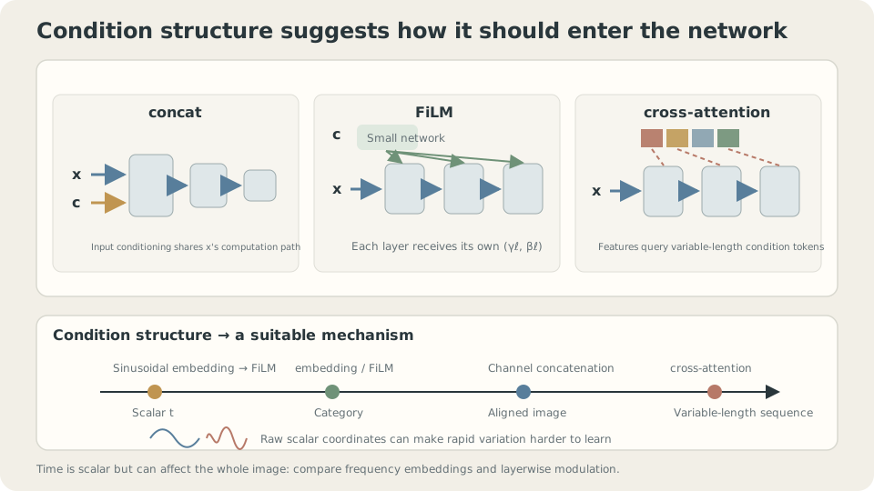
Figure: The three mechanisms change different computations. A time embedding is a representation choice for scalar conditions.

Why embed a scalar first?

A sinusoidal embedding maps $c\in[0,1]$ to multiple frequencies:

$$\mathrm{emb}(c)=\big(\sin(2\pi f_jc),\ \cos(2\pi f_jc)\big)_{j=0}^{J-1}, \qquad f_j=2^{\,j}.$$

It replaces “construct this oscillation from a scalar” with “use an oscillation already supplied in the input.”

For example, if $\sin(16\pi c)$ is already a feature, a linear layer can select it directly. This motivates Fourier features [2]; it does not imply that every network’s first-layer weights must grow as $O(k)$.

Check an important limitation: these integer frequencies give $\operatorname{emb}(0)=\operatorname{emb}(1)$. If the endpoints need different answers, retain raw $c$, include suitable noninteger frequencies, or use another endpoint-distinguishing representation.

Geometric frequencies $f_j=2^j$ cover several scales with only $J$ frequency pairs, or $2J$ trigonometric coordinates. Their ratio spans $2^{J-1}$ from the first frequency to the last.

SupplementThe link to positional encodings and Fourier features

Transformer sinusoidal positional encodings also use sine/cosine pairs at geometric frequencies. The scalar denotes token position rather than time or condition strength. The exact frequency choices and the way features enter the model differ.

Coordinate-based networks use related Fourier features [2]. Their neural-tangent-kernel analysis explains how feature mappings can alter a model’s effective spectral bias. The result depends on architecture and regime; it is not a theorem that all unembedded networks have exponentially decaying frequency response or can never learn high frequencies.

The reusable idea is to compare multiscale frequency features when a scalar must influence the output at several scales, while checking endpoint collisions and the frequencies the task actually needs.

Three representations on one task

Choose a target with deliberately rapid dependence on the condition:

$$y=\sin\big(2\pi x+2\pi\cdot 8\cdot t\big),\qquad x,t\sim U(0,1),\ n=800 .$$

The dependence on $x$ has one cycle, while the dependence on $t$ has eight. Run 6000 Adam steps at $\eta=0.01$ for each setting:

  concatenate scalar t          input dim  2   h= 64   training MSE 0.0018
  concatenate sinusoidal t      input dim 13   h= 64   training MSE 0.0004
  concatenate scalar t, wider   input dim  2   h=128   training MSE 0.0010

The embedding reduces displayed error by about a factor of four with 11 additional input coordinates. Doubling hidden width approximately quadruples the dominant hidden-layer parameter count, yet gives a smaller improvement here. This is evidence for this representation under this task and budget, rather than a universal efficiency ranking.

Fixed embedding frequencies need no training, but they change the representation, downstream parameter count, and represented functions. Controlled comparisons are needed to explain an improvement.

This motivates common sinusoidal time embeddings. They are part of the model’s input representation, even when the frequency map has no learned parameters. Like feature scaling in Downhill in Fog: Direction, Step Size, and Gradient Descent, they can change optimization, though their effect is more than a simple change of units.

“No condition” needs training too

A conditional model sometimes needs to operate without an explicit condition:

• To generate with no requested category.
• To compare conditional and unconditional predictions, as guidance methods often do.
• To handle a user who provides no condition.

A null token can represent absence—for example, an all-zero class vector. But if conditions are always present in training, that null input was never constrained by the objective.

Use $y=\sin(2\pi x)+0.8c$, with independent, equally likely binary classes. The unconditional squared-error predictor is therefore

$$\mathbb E[Y\mid X=x]=\sin(2\pi x)+0.4.$$

Independently replace the condition with null with probability $p$. Null examples then train this marginalized target. In general the average uses $p(c\mid x)$, not necessarily equal class weights.

def feats(x, c, mask):                      # mask=0 drops this condition
    oh = np.zeros((len(x), 2)); oh[np.arange(len(x)), c] = 1.0
    return np.c_[x, oh*mask[:,None]]

mask = (rng.random(N) > p).astype(float)    # p is condition-dropout probability

  dropout p=0.0   median null-prediction MSE against the class average: 1.3908
  dropout p=0.1   median null-prediction MSE against the class average: 0.0660
  dropout p=0.3   median null-prediction MSE against the class average: 0.0225
  reference: always predicting 0 gives MSE 0.6575

With $p=0$, the objective never constrains null behavior, and it performs poorly here. The function still has an output; there is no guarantee that it equals the class average. Other initializations or models need not fail by the same amount.

At $p=0.1$, null error falls by roughly twenty-one times; $p=0.3$ lowers it further. Increasing $p$ also reduces the fraction of condition-present examples. This table measures only null quality, so it cannot establish the conditional-quality tradeoff or an optimal dropout probability.

A null condition is an input whose desired behavior must be learned or otherwise specified.

A deliberate violation: replace the trained null vector with an unseen vector. Its behavior is again unconstrained and may be poor. The issue is not which vector looks geometrically neutral; use the null representation whose behavior the training objective actually specifies.

Limits of the experiment: these are small scalar/class-conditioned networks. For token sequences, dropping the entire condition and dropping individual tokens teach different tasks. Tune $p$ while measuring both conditional and null quality, since they share parameters. Independent dropout is important for the intended marginalization; selective missingness can change the null target.

Injection, frequency, and dropout

Interactive demo: Increase condition frequency and compare raw-scalar and embedded training curves. The embedding’s advantage depends on the supplied frequencies and training setup.

Check your understanding

Check your understanding

A model receives normalized scalar time, but its outputs at adjacent steps are almost identical. What should you do first? Immediately double the width. Check that neighboring steps require different answers and that time actually reaches the computation. Then compare raw time with an endpoint-distinguishing embedding. Similar adjacent outputs alone do not diagnose a frequency-learning failure. Use large unnormalized integer steps instead.

Show explanation

Check your understanding

A model was trained only with conditions present. At deployment, the team supplies an all-zero condition. What is guaranteed? The answer is the average of the two classes because zero is their midpoint. No class-average guarantee follows. The objective did not constrain null inputs; independent condition dropout is one way to train that branch. The model must choose exactly one of the classes.

Show explanation

Check your understanding

Which comparison of FiLM and concatenation is most reasonable? FiLM always wins because it influences every layer. Condition structure matters. Global class, time, or style can use feature modulation; an aligned mask or edge image naturally fits channelwise concatenation that preserves spatial correspondence. Concatenation always wins because it adds no parameters.

Show explanation

Check your understanding

Which statement is incorrect? Fixed sinusoidal frequencies need no learning, but change the input representation and downstream function class. Positional encodings and coordinate-network Fourier features both provide multiscale representations of scalar coordinates. Larger condition-dropout probability is always better because the null prediction becomes more accurate.

Show explanation

References

1. Perez, E. et al. FiLM: Visual Reasoning with a General Conditioning Layer. AAAI 2018.
2. Tancik, M. et al. Fourier Features Let Networks Learn High Frequency Functions in Low Dimensional Domains. NeurIPS 2020.
3. Ho, J., Salimans, T. Classifier-Free Diffusion Guidance. 2022.