L1.1 Ten Agents, Different Houses: Bias and Variance

Ten agents estimate the same house

Ten equally skilled agents use the same method but have seen different random samples of a hundred sales from one market.

Ask all ten to estimate the same new house. Their predictions form ten numbers.

How widely do they vary? A large spread indicates sensitivity to which training transactions were observed.

Is their average systematically wrong? If the mean estimate misses the conditional mean price, recruiting more identical-method agents does not remove that method’s average bias.

A method can be stable but biased, or correct on average but highly variable. These are distinct components requiring different investigations.

Should we measure average displacement or dataset-to-dataset fluctuation? Fix one query house and separate them.

Different components respond to different changes

• Irreducible risk $\mathbb E[\operatorname{Var}(Y\mid X)]$ is fixed for the chosen features and population. More training data does not change it, though additional informative features can change the prediction problem. Here it equals $0.0225$.
• Squared bias belongs to the whole learning procedure at the given sample size. Capacity, regularization, optimization, and finite data can all affect it; it is not simply approximation error.
• Prediction variance measures repeated-training fluctuations. It is not a synonym for estimation error. More data often helps, but arbitrary algorithms have no universal monotonic guarantee.

A high test score alone does not identify the dominant component. Investigate modeling and optimization for systematic bias, instability for variance, and improved features or uncertainty reporting when outcome noise dominates.

Averaging predictions can reduce variation when model errors are not perfectly correlated. It retains their common mean prediction, so a shared bias remains. For nonlinear networks, averaging parameters is different from averaging predictions and does not inherit this guarantee automatically.

Prediction averaging preserves the mean bias; variance reduction depends on correlation.

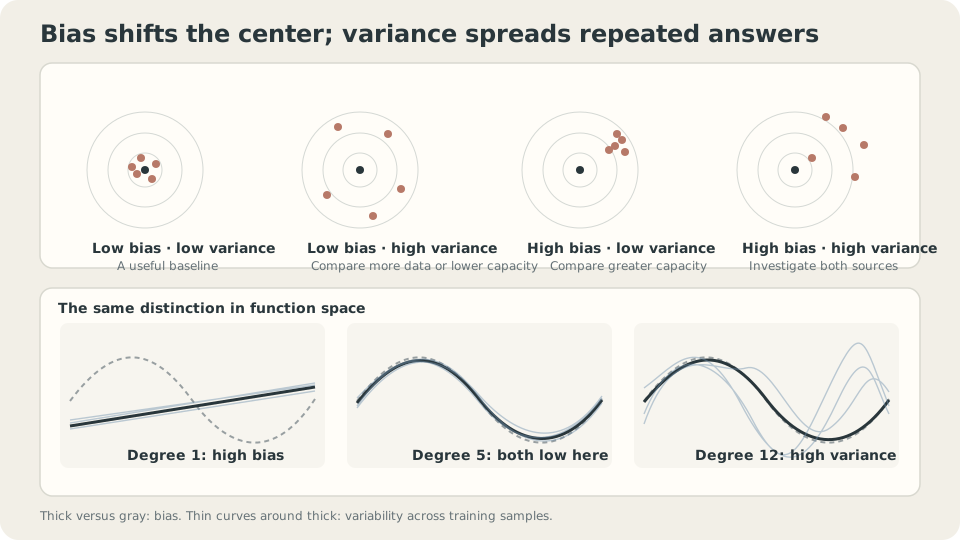
Bias compares the average fitted curve with truth; variance compares each fit with that average.

Derive the decomposition

At fixed $x$, abbreviate $\hat f=\hat f_D(x)$, $\bar f=\mathbb E_D\hat f$, and $f^\star=\mathbb E[Y\mid x]$. Split the error:

Square and average. Each cross term vanishes: the response residual is centered and independent of training randomness, and the estimator residual is centered over $D$. Hence

This repeats the orthogonality trick in Which Temperature Should We Forecast? MSE Selects the Conditional Mean, now with an extra layer of training-data randomness.

For fixed full-rank linear design, independent homoscedastic noise variance $\sigma^2$, and $k=d+1$ parameters, average fitted-prediction variance at the training inputs is

Within this setting, increasing parameter count at fixed design raises this average and increasing appropriate design size can reduce it. The formula does not automatically describe every test grid or nonlinear learning procedure.

Interventions and their limits

Widely varying estimates: compare more relevant data, suitable restrictions, regularization, and prediction ensembling. Their effectiveness depends on the source of variation.

Consistent systematic error: inspect missing features and model or optimization restrictions. Averaging more same-law predictions does not change their common mean; more training data can still change the underlying procedure’s bias, so its effect needs checking.

Accurate conditional mean but variable outcomes: report suitable uncertainty or seek features explaining the remaining variability. A point estimator cannot predict independent residual noise.

Repeated-training estimates need representative resampling and enough replications. Shared or correlated datasets alter uncertainty in the estimates. The formula assumes a fresh independent response and squared loss.

Measure the components

Fix thirty input locations and resample only response noise, fitting three hundred datasets per degree:

import numpy as np
from numpy.polynomial import Polynomial
from ml_toy import truth, NOISE
xs,ys = truth()
x = np.linspace(0,1,30)
Y = np.sin(2*np.pi*x)+NOISE*np.random.default_rng(0).standard_normal((300,30))
for d in (1,2,3,5,7,9,12):
    P = np.array([Polynomial.fit(x,yy,d)(xs) for yy in Y])
    bias2 = ((P.mean(0)-ys)**2).mean()
    var = P.var(0).mean()
    print(d,'bias squared',bias2,'variance',var,'noise',NOISE**2,'sum',bias2+var+NOISE**2)

degree  bias²   variance  noise   sum
1       0.2004  0.0016    0.0225  0.2245
2       0.2004  0.0022    0.0225  0.2251
3       0.0048  0.0028    0.0225  0.0301
5       0.0000  0.0041    0.0225  0.0266
7       0.0000  0.0053    0.0225  0.0278
9       0.0000  0.0069    0.0225  0.0294
12      0.0000  0.0095    0.0225  0.0320

In this experiment, squared bias falls sharply while variance rises, producing the observed risk minimum near degree five. Values rounded to zero are not a proof of exact zero bias. The decomposition is exact; a U-shaped trend as capacity varies remains a property of the procedure and setting.

Read three features of the table:

• Degrees one and two have similar bias at the displayed precision; the added term helps little here.
• Beyond degree five, small additional approximation gains are outweighed by measured variance in this comparison.
• Outcome noise stays fixed at $0.0225$ because the data-generating problem is unchanged.

Check the scale: keep degree nine and vary the fixed input-grid size:

for n in (30,100,300):
    x = np.linspace(0,1,n)
    Y = np.sin(2*np.pi*x)+NOISE*np.random.default_rng(0).standard_normal((300,n))
    P = np.array([Polynomial.fit(x,yy,9)(xs) for yy in Y])
    print(n,'grid variance',P.var(0).mean(),'training-input formula',NOISE**2*10/n)

n=30:  grid variance 0.0069, training-input formula 0.0075
n=100: grid variance 0.0021, training-input formula 0.0022
n=300: grid variance 0.0008, training-input formula 0.0007

The dense-grid average happens to be similar in scale, but its exact conditional variance averages $\sigma^2\phi(x)^\top(V^\top V)^{-1}\phi(x)$ over that grid. Only averaging at the original training inputs gives exactly $\sigma^2k/n$.

More data can change the entire estimator; only the irreducible risk of a fixed prediction problem is independent of training size.

With zero noise and fixed inputs, deterministic fitting has no repeated-noise variance. Resampling input locations introduces design randomness, which can still change predictions without label noise. Whether it causes large fluctuations in this particular toy must be measured, not assumed.

Explore the components

Specify the resampling experiment before interpreting how data and capacity change the components.

Check your understanding

References

1. Geman, S., Bienenstock, E., Doursat, R. Neural Networks and the Bias/Variance Dilemma. Neural Computation 1992.
2. Hastie, T., Tibshirani, R., Friedman, J. The Elements of Statistical Learning, 2nd ed. Springer 2009, Ch. 7.3.
3. Domingos, P. A Unified Bias-Variance Decomposition and its Applications. ICML 2000.