M5.0 Why Insurance Can Make Sense: Convexity and Jensen's Inequality

Why pay more than the average loss?

In a simplified mathematical insurance model, a yearly loss is 200,000 with probability 0.02 and zero otherwise. A premium of 6,000 fully covers it. The expected loss is 4,000, below the premium.

Yet a certain expense of 6,000 may have less impact than an occasional sudden loss of 200,000. Are we comparing amounts or their consequences? Represent the consequence by a function first.

A chord above a curve

Increasing marginal disutility produces an upward-bending, bowl-like curve.

Join its points at losses zero and 200,000. The chord at 4,000, two percent of the way across, has height $\mathbb E[\varphi(X)]$. The curve itself has height $\varphi(\mathbb E[X])$.

For a convex curve, the chord lies above it. This gives $\mathbb E[\varphi(X)]\ge\varphi(\mathbb E[X])$. Their vertical separation is the Jensen gap.

This compares an uncertain loss with a certain loss of 4,000. To justify the actual premium, separately check $\varphi(6000)\le\mathbb E[\varphi(X)]$. Jensen alone does not establish that comparison.

Pooling independent identical losses reduces variance of the per-person mean to $\operatorname{Var}(X)/n$. This does not guarantee an insurer’s profit; dependence, costs, and coverage terms also matter.

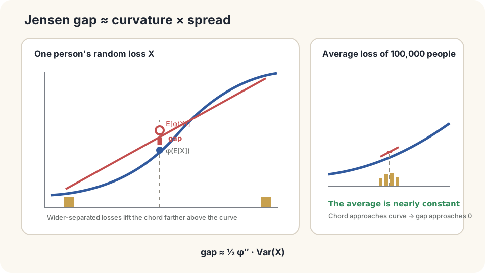
The Jensen gap depends jointly on curvature and the input distribution.

Convexity and Jensen

A function $\varphi$ on a convex domain is convex if, for any $a,b$ and $\lambda\in[0,1]$,

The left side is a curve value; the right side is the chord value. For twice-differentiable functions on an interval, convexity is equivalent to $\varphi''\ge0$. Examples include $x^2$, $e^x$, and $-\log x$ on their domains. Logarithm and square root are concave, reversing the shape.

Jensen’s inequality: for convex $\varphi$ under appropriate integrability,

Proof. Let $m=\mathbb E[X]$ lie inside the domain and choose a supporting line $\ell(x)=\varphi(m)+c(x-m)$ below the curve. If differentiable, $c=\varphi'(m)$. Taking expectations gives

Only the supporting-line inequality and linearity of expectation were needed. Two-point convexity is the special case of Jensen for a two-valued variable.

Equality requires $\varphi(X)=\ell(X)$ almost surely. For strictly convex $\varphi$, the supporting line meets the curve only at $m$, so equality holds exactly when $X$ is almost surely constant.

For a concentrated variable, expand to second order around $m$ and average. The linear term vanishes:

This is a local approximation requiring control of higher-order remainders. If the entire relevant interval satisfies $0\le m_2\le\varphi''\le M_2$, Taylor’s integral remainder instead gives rigorous bounds:

Variance alone does not order arbitrary Jensen gaps. Curvature and distributional shape also matter.

Return to the premium

The actual comparison is $\varphi(6000)$ versus expected uninsured disutility. Once $\varphi$ is chosen, calculate both. Jensen explains the averaging distinction; it does not choose a person’s preferences.

Check the assumptions:

• Convexity on the relevant domain: a capped or nonconvex consequence function need not obey the same direction. Its shape alone still does not settle every premium comparison.
• Defined expectations: heavy tails can make a mean infinite or an expression undefined, so ordinary finite-gap reasoning cannot be applied unchanged.

Simulate, then reverse the curvature

import numpy as np
rng = np.random.default_rng(0)
loss = np.where(rng.random(200000)<.02,200000.,0.)
phi = lambda x:-np.log1p(-x/250000)
print('mean loss:',loss.mean())
print('premium disutility and expected loss disutility:',phi(6000.),phi(loss).mean())
pool = loss.reshape(2,100000).mean(1)
print('pooled means and empirical gap:',pool,phi(pool).mean()-phi(pool.mean()))
phi_c = np.sqrt
print('concave comparison:',phi_c(4000.),phi_c(loss).mean())

For this chosen convex function, the premium’s disutility is smaller than expected uninsured disutility. Large independent pools have much more concentrated per-person means. With $\sqrt x$, the Jensen direction reverses: $\sqrt{4000}\approx63.2$, while $0.02\sqrt{200000}\approx8.9$. Preference and premium comparisons still require the actual two costs.

Vary curvature, spread, and pool size to compare $\mathbb E[\varphi(X)]$ with $\varphi(\mathbb E[X])$.

Check your understanding

References

1. Boyd, S., Vandenberghe, L. Convex Optimization. Cambridge University Press, 2004.
2. Jensen, J. L. W. V. Sur les fonctions convexes et les inégalités entre les valeurs moyennes. Acta Mathematica 30, 1906.
3. Cover, T. M., Thomas, J. A. Elements of Information Theory. Wiley, 2nd ed., 2006.
4. Grimmett, G., Stirzaker, D. Probability and Random Processes. Oxford University Press, 3rd ed., 2001.