M1.0 Two Scales: Linear Combinations of Gaussians

Two readings

Two unbiased scales have noise standard deviations 1 kg and 0.5 kg. Today they read 72.8 and 71.9 kg.

Which weight should you report?

Using both sounds useful, but equal weighting might let the noisier scale undermine the better one.

Treat the quoted noise magnitudes as standard deviations, not guaranteed error limits. Minimize the variance of an unbiased weighted combination.

DiscussionQ1

What is random, how do we represent reliability, and which estimators are being compared?

Show the reasoning

The true weight $w$ is fixed but unknown. The readings are random.

Write $Y_A=w+\varepsilon_A$ and $Y_B=w+\varepsilon_B$ , with zero-mean independent errors of known variances. Gaussian errors additionally specify their full distribution.

Compare $\hat w=aY_A+bY_B$ . Unbiasedness requires $a+b=1$ . Equal averaging and using only scale B are special cases. We seek the lowest-variance estimator in this linear unbiased family.

Combine two independent jitters

Two independent displacements sometimes reinforce and sometimes oppose each other. Their variances add: standard deviations 1 and 0.5 combine to $\sqrt{1^2+0.5^2}\approx1.12$ , rather than their sum or maximum.

Gaussianity additionally preserves the bell-shaped distribution under linear combination.

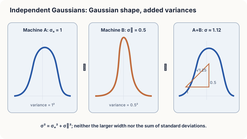
Independent Gaussian errors combine by adding variances while retaining Gaussian form.

Figure: standard deviations combine through their squares.

Write the combination mathematically

A scalar Gaussian has density $\exp(-(x-\mu)^2/(2\sigma^2))/(\sqrt{2\pi}\sigma)$ . Two useful rules are:

Affine transformation: $aX+b\sim\mathcal N(a\mu+b,a^2\sigma^2)$ .
Independent addition: Gaussian means and variances each add.

For independent Gaussian linear combinations, means use the coefficients and variances their squares. Variance addition itself only needs uncorrelated finite-variance errors; Gaussianity identifies the resulting distribution.

DetailsProve Gaussian closure using moment-generating functions

The Gaussian MGF is $M_X(s)=\exp(\mu s+\sigma^2s^2/2)$ . Independence factors the MGF of a sum:

M_{X_1+X_2}(s)=\exp\!\big((\mu_1+\mu_2)s+\tfrac12(\sigma_1^2+\sigma_2^2)s^2\big),

This is the MGF of the stated Gaussian. In general, sum variance includes twice the covariance, which vanishes under independence.

Vectors. The covariance matrix stores individual variances on its diagonal and pairwise covariance elsewhere. An affine transformation of a multivariate Gaussian satisfies

AX+b\sim\mathcal N\big(A\mu+b,\ A\Sigma A^{\!\top}\big).

A weighted scalar estimate has variance $a^\top\Sigma a$ , reducing to $\sum_i a_i^2\sigma_i^2$ for independent coordinates.

Equal averaging or reliability weighting?

For an unbiased combination with independent errors,

\mathrm{Var}(\hat w)=a^2\sigma_A^2+b^2\sigma_B^2 .

The cross term vanishes, and squared weights determine each variance contribution.

Equal average: variance 0.3125 and standard deviation about 0.559 kg.
Only B: variance 0.25 and standard deviation 0.5 kg.

Equal averaging is worse than using only B. The information is useful, but the assigned weights are poor.

Differentiate the variance with respect to $a$ , setting $b=1-a$ :

a=\frac{1/\sigma_A^2}{1/\sigma_A^2+1/\sigma_B^2},\qquad b=\frac{1/\sigma_B^2}{1/\sigma_A^2+1/\sigma_B^2},\qquad \mathrm{Var}(\hat w)=\frac{1}{1/\sigma_A^2+1/\sigma_B^2}.

Weights are proportional to precision, or inverse variance. Here $a=0.2$ , $b=0.8$ , the estimate is 72.08 kg, and its standard deviation is about 0.447 kg. Independent precisions add; the same rule extends to more measurements.

This optimizes linear unbiased estimation under the stated known variances. The weight calculation does not require Gaussianity, and does not claim optimality among every possible biased estimator at every parameter value.

Correlated errors require covariance terms. With a shared independent error $c$ , averaging $n$ devices leaves variance $\sigma_c^2+\sigma^2/n$ : the common component remains. Bias or outliers require checking the error model again.

Simulate ten thousand mornings

import numpy as np
rng = np.random.default_rng(0); n = 10_000; w = 72.0
sA, sB = 1.0, 0.5
def trial(rho=0.0, glitch=0.0):
    eA = rng.normal(0, sA, n)
    eB = rho*eA*(sB/sA) + np.sqrt(1-rho**2)*rng.normal(0, sB, n)
    eA = eA + glitch*rng.choice([0, 10], n, p=[0.98, 0.02])
    yA, yB = w + eA, w + eB
    for name, est in [("mean", (yA+yB)/2), ("B", yB), ("weighted", 0.2*yA+0.8*yB)]:
        print(name, "standard deviation", est.std())
for rho, g in [(0.0, 0), (0.8, 0), (0.0, 1)]:
    print(rho, g); trial(rho, g)

The independent case matches the derived standard deviations. Correlation invalidates weights that ignore covariance; glitches change the actual variance and may introduce bias. These are reasons to update the error model, not to reject all non-Gaussian linear combinations.

Check your understanding

References

Grimmett, G., Stirzaker, D. Probability and Random Processes, 3rd ed. Oxford University Press 2001.
Bishop, C. M. Pattern Recognition and Machine Learning. Springer 2006, Ch. 2.3.
Kay, S. M. Fundamentals of Statistical Signal Processing, Vol. I: Estimation Theory. Prentice Hall 1993.