
L1.0 Memorizing Old Exams: Overfitting and Underfitting
Builds on2 notes
Two students with the same poor score
Two students both score forty on an exam.
One memorized every past answer and scores perfectly when old questions repeat, but struggles when the numbers change.
The other carefully studied only half the material, scoring forty-five on practice questions and forty on the exam.
Their final scores hide different problems: memorizing particular examples versus lacking sufficient knowledge. Remedies therefore require evidence about what each student learned, not just the final score.
Practice performance adds useful information: 100/40 differs from 45/40.
Likewise, training and fresh-example errors should be examined together.
One score is insufficient for diagnosing generalization.
How can the two scores guide learning a transferable rule? First identify plausible causes, then vary capacity and sample size in the same toy.
Two students score forty.
Who memorized answers, and who has not learned enough?
Relative to what is a model too complex?
DiscussionQ1
List the combinations of small or large training and population risks. What do they suggest checking?
Show the reasoning
Use training risk and population risk from A Property Agent Moves Cities: Risk and Empirical Risk. Memorization can produce low training risk and high population risk; insufficient fitting can leave both high.
| Small population risk | Large population risk | |
|---|---|---|
| Small training risk | Desired performance | Investigate overfitting, data quantity, and regularization |
| Large training risk | Check sampling and evaluation consistency | Check capacity, features, and optimization |
All four combinations can occur. Training augmentation, dropout, penalties, harder examples, and sampling fluctuations affect comparability. Recompute both scores with the same evaluation mode and loss before interpreting the gap.
Remedies can conflict: stronger restrictions can worsen capacity limitations, while additional unconstrained capacity may worsen memorization. Neither outcome is guaranteed from capacity alone; compare the actual intervention.
Capacity can fail in different ways
Polynomial degree, tree depth, network width, and regularization affect effective flexibility, though they are not interchangeable complexity measures.
- Underfitting: the family cannot approximate the relevant pattern, or the procedure has not found a sufficiently good fit. Both scores can stay high.
- Overfitting: fitting sample-specific variation improves the training score without comparable fresh-example improvement. Estimation effects can dominate.
The useful capacity depends jointly on model, data amount, algorithm, and regularization. When someone says “too complex,” ask for which dataset and training procedure?
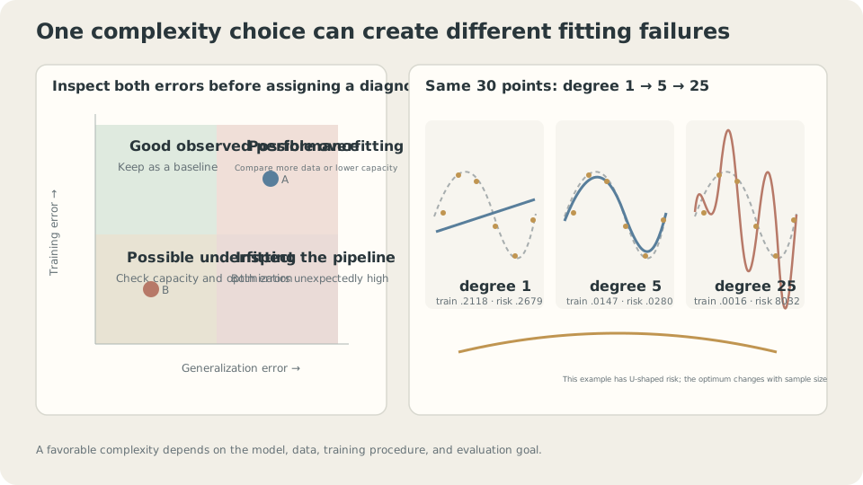
Capacity limitations and sample-specific fitting require different checks; useful flexibility depends on available data.
Why a U-shaped curve can appear
For fixed data and nested families , exact ERM gives one guaranteed direction:
- Minimum training risk cannot increase when the feasible family expands.
- Population risk includes approximation, estimation, and irreducible components. Approximation improves or stays equal, but estimation need not change monotonically. A classical U shape is common, not a theorem following from nesting alone [1].
More independent data can reduce estimation uncertainty and permit more flexibility. The curve can flatten and its best setting can move, but these are qualitative patterns to check rather than universal sample-by-sample laws.
Some overparameterized models exhibit double descent, with another decrease after an interpolation-region peak [2]. This is a phenomenon under particular models and algorithms, not a promise from increasing capacity. The displayed polynomial experiment stays below its sample count.
Under squared loss, the population optimum is , with irreducible risk . Here that is , a reference for population performance rather than a hard training-loss floor.
CautionA positive loss plateau need not be a capacity failure
Does a nonzero plateau mean more layers are necessary?
Compare with the same task’s irreducible population MSE, independent validation, and useful baselines. A finite training score can fall below the noise level; stopping near it also does not automatically prove success.
Repeated measurements at fixed input can estimate conditional noise. Expert agreement and known synthetic mechanisms can offer other reference information, with their respective limitations. Without a relevant baseline, a plateau at 0.3 is difficult to interpret.
Choose a remedy from evidence
Overfitting: try appropriate restrictions, more relevant independent data, justified augmentation, regularization, or early stopping; see Limit the Notes or Stop Practicing: Regularization and Early Stopping. These are interventions to compare, not automatic cures.
Insufficient fitting: consider richer informative features, suitable capacity, or better optimization. In Downhill in Fog: Direction, Step Size, and Gradient Descent, a tiny rate left a capable model poorly optimized.
A small-subset fitting test can expose implementation, capacity, or optimization difficulties: can the system fit a manageable subset under permissive settings? Success shows that particular test is feasible; it does not prove the full-data pipeline or generalization is correct. Failure also requires checking labels, constraints, and the objective.
Evaluation must use independent appropriate data with consistent scoring. Distribution shift can create another gap. Nested-family intuition does not transfer unchanged between unrelated architectures and algorithms.
Observe the curve, then add data
For thirty shared toy observations, vary polynomial degree:
import numpy as np
from numpy.polynomial import Polynomial
from ml_toy import toy_1d, truth, NOISE
xs, ys = truth()
risk = lambda f:((f(xs)-ys)**2).mean()+NOISE**2
x,y = toy_1d()
for d in (0,1,2,3,5,7,9,12,15,20,25):
    f = Polynomial.fit(x,y,d)
    print(d,'training',((f(x)-y)**2).mean(),'population approximation',risk(f))
degree training population approximation
0 0.3897 0.5575
1 0.2118 0.2679
2 0.2117 0.2668
3 0.0178 0.0312
5 0.0147 0.0280
7 0.0134 0.0296
9 0.0122 0.0285
12 0.0114 0.0314
15 0.0104 0.0334
20 0.0043 0.0659
25 0.0016 8032.3199Training risk decreases, while population risk first drops and later grows dramatically, with small local fluctuations. A line misses the sine pattern. High degrees fit observed noise yet perform poorly elsewhere. Read the two scores together; no universal ratio threshold diagnoses underfitting.
Adding a quadratic term barely helps this example; a cubic captures much more of the sine shape. Additional capacity matters through which functions it enables, not just parameter count.
Now use three hundred observations:
x3,y3 = toy_1d(n=300,seed=1)
for d in (1,3,9,15,20,25):
    f = Polynomial.fit(x3,y3,d)
    print(d,'training',((f(x3)-y3)**2).mean(),'population approximation',risk(f))
degree training population approximation
1 0.2106 0.2207
3 0.0266 0.0277
9 0.0198 0.0242
15 0.0197 0.0243
20 0.0196 0.0244
25 0.0194 0.0283The disastrous high-degree behavior is greatly reduced in this sample. Degrees nine through twenty stay near the population noise floor. Degree twenty-five still worsens somewhat, so the curve has flattened rather than establishing that additional capacity can never hurt.
Thus “degree twenty-five always overfits” is unsupported. Its behavior depends on the observations, training procedure, and evaluation distribution.
Judge capacity relative to data and training conditions.
Large datasets are one reason highly flexible models can work. Architecture, regularization, optimization, and task structure also matter; data amount alone does not explain every modern result.
Removing noise makes the irreducible risk zero but does not guarantee accurate unseen predictions. Thirty distinct inputs uniquely determine the degree-twenty-five least-squares solution in exact arithmetic; uniqueness is different from correctness between inputs.
Vary data quantity and capacity
Compare the capacity curves at different sample sizes rather than treating complexity as an absolute verdict.
Check your understanding
References
- Hastie, T., Tibshirani, R., Friedman, J. The Elements of Statistical Learning, 2nd ed. Springer 2009, Ch. 7.
- Belkin, M. et al. Reconciling modern machine-learning practice and the classical bias–variance trade-off. PNAS 2019.
- Ng, A. Machine Learning Yearning 2018, Ch. 20–27.