M5.1 The Cost of a Wrong Probability Table: KL Divergence and Cross-Entropy

Builds on2 notes

A wrong weather table

Consider a mathematical betting model with sunny, rainy, and cloudy outcomes. A bookmaker’s positive table $b$ sets payout multipliers $1/b(x)$ . Each participant allocates all wealth among outcomes.

This is a probability illustration. If someone believes table $q$ , allocating in proportions $q$ maximizes expected log wealth under that belief [3]. But actual outcomes follow another table $p$ .

Compare two people observing the same outcomes, using allocations $p$ and $q$ . Wealth multiplies, so logarithms turn the accumulated comparison into a sum.

DiscussionQ1

Define daily outcomes and wealth updates. Which quantity measures the cost of using the wrong table?

Show the reasoning

Let iid $X_t\sim p$ . Allocating by $q$ multiplies wealth by $q(X_t)/b(X_t)$ each day. Under integrability,

W_n=W_0\prod_{t=1}^n\frac{q(X_t)}{b(X_t)},\qquad \frac1n\log\frac{W_n}{W_0}=\frac1n\sum_{t=1}^n\log\frac{q(X_t)}{b(X_t)} \longrightarrow\mathbb E_p\!\left[\log\frac{q(X)}{b(X)}\right].

The logarithm turns compounding into addition. The expectation is under true outcome law $p$ , regardless of the participant’s belief.

Subtract this expected log growth from that obtained with allocation $p$ :

\mathbb E_p\!\left[\log\frac{p(X)}{b(X)}\right]-\mathbb E_p\!\left[\log\frac{q(X)}{b(X)}\right] =\mathbb E_p\!\left[\log\frac{p(X)}{q(X)}\right].

The common payout table cancels. Expected annual log-wealth difference is 365 times this value; a realized year still fluctuates.

A small expected cost each day

On a logarithmic wealth plot, both realized paths fluctuate, but their expected slopes differ by a fixed amount.

The expected gap grows linearly. The actual gap need not increase by the same amount every day, or even increase every day.

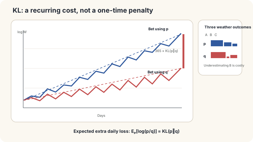
Accumulating expected log cost from using a wrong probability table.

Realized log differences fluctuate; their expectation accumulates at rate $\mathrm{KL}(p\|q)$ .

KL, nonnegativity, and cross-entropy

For distributions on the same sample space, define Kullback–Leibler divergence:

\mathrm{KL}(p\,\|\,q)=\sum_x p(x)\log\frac{p(x)}{q(x)}=\mathbb E_{X\sim p}\Big[\log\frac{p(X)}{q(X)}\Big].

Use an integral for densities. A zero- $p$ term contributes zero; positive $p$ where $q=0$ gives infinite KL. Interpret it as excess expected log cost when observations follow $p$ but predictions use $q$ [2].

Nonnegativity. Write KL as $-\mathbb E_p[\log(q/p)]$ . Convexity of $-\log$ and Jensen give

-\mathbb E_p\Big[\log\frac{q(X)}{p(X)}\Big]\ge-\log\sum_{x:p(x)>0}q(x)\ge-\log1=0.\qquad\square

Equality in Jensen requires $q/p$ constant on the support of $p$ ; equality in the normalization step requires no extra $q$ mass outside it. Together they give $p=q$ . KL vanishes exactly for identical laws, but is not a metric.

Entropy and cross-entropy. Split the log ratio:

\mathrm{KL}(p\,\|\,q)=\underbrace{\mathbb E_p[-\log q(X)]}_{H(p,q)\ \text{cross-entropy}}-\underbrace{\mathbb E_p[-\log p(X)]}_{H(p)\ \text{entropy}}.

When these quantities are finite, cross-entropy is the correct-table cost plus excess cost. For fixed $p$ , minimizing it is equivalent to minimizing KL. Differential entropy for continuous densities can be negative and has a different interpretation from discrete entropy.

Asymmetry matters: generally $\mathrm{KL}(p\|q)\ne\mathrm{KL}(q\|p)$ .

If $p(x)>0$ remains fixed while $q(x)\to0$ , the contribution grows without bound: a true event is severely underpredicted.
If $p(x)=0$ , its direct contribution vanishes. Allocating $q$ mass there still removes mass from other outcomes and can increase the total cost.

Reversing the arguments changes the averaging law. $\mathrm{KL}(q\|p)$ is infinite when $q$ places positive mass where $p=0$ . This direction treats errors differently; neither direction is universally the larger number.

DetailsNot a metric, but additive for independent products

KL is asymmetric and does not satisfy a metric triangle inequality. For independent product laws, $\mathrm{KL}(p_1p_2\|q_1q_2)=\mathrm{KL}(p_1\|q_1)+\mathrm{KL}(p_2\|q_2)$ : split the logarithm and take expectations.

Pinsker’s inequality with natural logarithms gives KL(p‖q)≥½‖p−q‖₁². Thus small KL controls every event-probability difference. The converse fails: small total variation can coexist with infinite KL through a support mismatch.

Quantify the asymmetry

For $p=(0.5,0.3,0.2)$ and $q=(0.6,0.1,0.3)$ , calculate

\mathrm{KL}(p\|q)=0.5\log\frac{0.5}{0.6}+0.3\log\frac{0.3}{0.1}+0.2\log\frac{0.2}{0.3}\approx0.158\ \text{nats per day}.

The annual expected log gap is about 57.4 nats. This is neither a deterministic wealth ratio nor the logarithm of an expected wealth ratio. Individual summands can be negative; only the total is guaranteed nonnegative.

Swapping the two tables gives approximately $0.121$ , rather than $0.158$ . The same absolute probability discrepancy can have different log costs depending on the true law.

The long-run sample-average statement assumes fixed iid outcomes and an integrable log ratio. Keeping some wealth unallocated changes the multiplier and does not simply scale KL by the allocated fraction.

Simulate a year and nearly remove an outcome

import numpy as np
rng = np.random.default_rng(0)
p = np.array([.5,.3,.2])
q = np.array([.6,.1,.3])
kl = lambda a,b:np.sum(a*np.log(a/b))
print(kl(p,q),kl(q,p))
x = rng.choice(3,size=(2000,365),p=p)
gap = np.log(p[x]).sum(1)-np.log(q[x]).sum(1)
print('daily mean and annualized fluctuation:',gap.mean()/365,gap.std()/365)
q_bad = np.array([.7,1e-6,.3-1e-6])
print('near-zero rainy probability:',kl(p,q_bad))

The simulated daily expected gap approaches $0.158$ , with finite-year fluctuations. Making rainy probability $10^{-6}$ raises KL to about 3.5 nats per observation. The formula identifies which underpredicted events dominate the cost.

Change $q$ and exchange the two arguments to inspect the costly errors.

Check your understanding

References

Cover, T. M., Thomas, J. A. Elements of Information Theory. Wiley, 2nd ed., 2006.、
Kullback, S., Leibler, R. A. On Information and Sufficiency. Annals of Mathematical Statistics 22(1), 1951.
Kelly, J. L. A New Interpretation of Information Rate. Bell System Technical Journal 35(4), 1956.
MacKay, D. J. C. Information Theory, Inference, and Learning Algorithms. Cambridge University Press, 2003.