L2.3 Limit the Notes or Stop Practicing: Regularization and Early Stopping

Builds on2 notes

Two interventions against memorization

Return to the student memorizing old exams in Memorizing Old Exams: Overfitting and Underfitting.

Limit the notes: one handwritten page encourages compact rules rather than storing every answer.

Limit practice time: stop before excessive attention to particular question details.

Both restrictions can remove irrelevant detail or prevent useful learning. Which solutions do they restrict mathematically? A linear model makes their effects explicit.

How can limiting parameters and limiting time have similar effects?
When do their predictions differ?
How do we decide whether either restriction helps?

DiscussionQ1

Write a parameter penalty, derive its solution, and explain when smaller parameters control function variation.

Show the reasoning

Add a quadratic parameter penalty to the empirical objective:

\frac{1}{2n}\lVert Vw-y\rVert^2+\frac{\lambda}{2}\lVert w\rVert^2 .

The coefficient $\lambda$ trades training fit for smaller parameter norm. Half factors simplify differentiation. If all coordinates are penalized, increasing the coefficient toward infinity drives parameters toward zero.

For linear least squares with $H=V^\top V/n$ , stationarity gives

(H+\lambda I)\,w=\frac1nV^\top y \quad\Longrightarrow\quad w_\lambda=(H+\lambda I)^{-1}\tfrac1nV^\top y .

Project onto an eigenvector with eigenvalue $\mu_j$ :

w_\lambda^{(j)}=\frac{\mu_j}{\mu_j+\lambda}\cdot w_{0}^{(j)},

Relative to a least-squares solution in positive-curvature directions, the factor $\mu_j/(\mu_j+\lambda)$ strongly suppresses weak directions and preserves strong ones. Null directions require choosing an appropriate least-squares reference.

For fixed differentiable features, $|f_w'(x)|\le\|w\|\|\phi'(x)\|$ . Norm control can therefore bound variation in that representation, but depends on feature scales. Small curvature means the training objective changes weakly along a direction, not that all values along it are equally good.

Starting GD at zero also learns stronger-curvature directions earlier under a nonoscillatory stable step. That gives a related filtering effect, though not the same parameter path.

Three kinds of restriction

Compare what each operation changes:

Ridge/L2 penalty: changes the objective and gives the stated linear spectral filter. Direct weight decay equals this update for ordinary GD under matched conventions, not every optimizer.
Early stopping: limits the duration of optimization, yielding filter $1-(1-\eta\mu_j)^t$ in the linear zero-start setting.
Dropout: randomly masks units during training. Particular linear squared-loss settings admit a scale-dependent penalty interpretation; deep-network behavior is more complex than an exact ensemble average.

Such changes can trade bias for lower variation in simple settings. General networks have no universal monotonic tradeoff or guaranteed validation improvement.

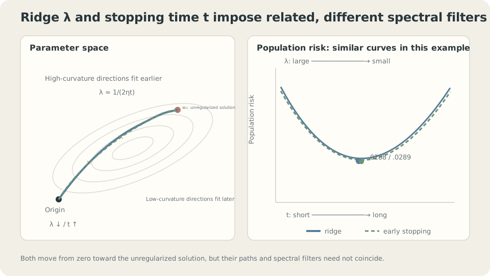
Ridge and early stopping filter weak directions differently.

Both can suppress weak feature directions, but their trajectories and filters differ.

Compare the filters

In the eigenbasis of fixed $H$ , compare the fraction of the least-squares solution retained.

Ridge:

q_j^{\mathrm{ridge}}=\frac{\mu_j}{\mu_j+\lambda}.

GD after $t$ updates from zero: each error component multiplies by $1-\eta\mu_j$ , so

q_j^{\mathrm{GD}}=1-(1-\eta\mu_j)^t\approx1-e^{-\eta\mu_jt}.

For $0<\eta\le1/\mu_{\max}$ , these filters increase nonoscillatorily from zero. Small $\eta\mu_j$ permits the exponential approximation. Transition scales are approximately $\mu_j\sim\lambda$ and $\mu_j\sim1/(\eta t)$ , giving

\boxed{\ \lambda\approx\frac{1}{\eta t}\ }

$\lambda\approx1/(\eta t)$ aligns scales, not every eigendirection exactly.

Stopping count and rate must be interpreted together. A schedule replaces the constant-rate power by a product of step-specific factors. Explicit penalties and stopping can coexist, but their combined improvement requires validation.

DetailsWhy aligned scales do not imply identical solutions

For small curvature, the filters behave like μ/λ and ημt. At large curvature, ridge approaches one algebraically while the exponential approximation approaches it exponentially. Matching one transition scale cannot match the whole spectrum.

The example below finds similar best risks for ridge and stopping while their early-trajectory risks differ. This illustrates related filtering without establishing identical parameters.

Other datasets need not have equally close best risks or equally broad good regions. Examine validation sensitivity rather than assuming a universal flat optimum.

CautionAdaptive scaling changes the meaning of decay

Adding $\lambda w$ to Adam’s gradient sends the penalty through its adaptive moment processing. This differs from applying direct parameter shrinkage after the adaptive loss-gradient step.

AdamW decouples the two:

w\leftarrow w-\eta\,\frac{\hat m}{\sqrt{\hat s}+\epsilon}-\eta\lambda w .

Consequently the same numerical coefficient does not imply the same effective regularization across optimizers and conventions. See One Learning Rate Is Not Enough: Momentum and Adam.

When should restrictions help?

Low training and high validation errors motivate testing restrictions. Two high errors motivate checking capacity, data, objective, and optimization first. Those patterns are clues, not a measured bias–variance decomposition.

Compare a modest range of strengths on the same development protocol. Selecting a stopping point also uses validation data and needs independent final evaluation. Combining restrictions is possible without a universal ordering of optimal strengths.

The spectral derivation assumes linear features, squared loss, and the stated initialization/rate. Nonlinear networks do not inherit its exact filters. L2 also depends on parameterization and feature scale. Intercepts are often excluded from penalties, but that is a modeling choice to specify rather than a mathematical prohibition.

Compare two regularization paths

Use thirty examples and degree-twenty polynomial features. Maximum-column scaling is not centered unit-variance standardization. Raw normal equations remain ill-conditioned; use stable augmented least squares for the comparison below.

Ridge sweep:

import numpy as np
from ml_toy import toy_1d, truth, NOISE
xs,ys = truth()
x,y = toy_1d(n=30,seed=0)
n,D = len(x),20
mx = np.abs(np.vander(np.linspace(0,1,80),D+1,increasing=True)).max(0)
B = lambda X:np.vander(X,D+1,increasing=True)/mx
A,As = B(x),B(xs)
risk = lambda w:((As@w-ys)**2).mean()+NOISE**2
for lam in (0,1e-8,1e-6,1e-4,1e-3,1e-2,.1,1,10):
    aug = np.vstack([A,np.sqrt(lam*n)*np.eye(D+1)])
    target = np.r_[y,np.zeros(D+1)]
    w = np.linalg.lstsq(aug,target,rcond=None)[0]
    print(lam,'training',((A@w-y)**2).mean(),'population',risk(w))
# Stable arithmetic can differ from ill-conditioned normal-equation records below.

Original normal-equation experiment record:
lambda  training   population
0       .0106      .0321
1e-8    .0129      .0288
1e-6    .0134      .0292
1e-4    .0208      .0406
1e-3    .0578      .0831
.01     .1246      .1709
.1      .1898      .2902
1       .3139      .4439
10      .3929      .5001

The selected small penalty helps this record, while larger penalties suppress useful directions. For exact ridge solutions, increasing the coefficient makes parameter norm nonincreasing and unpenalized training loss nondecreasing, allowing ties. Numerical results need solver checks before using those monotonic properties as diagnostics.

Early stopping: use the same family with zero explicit penalty.

w = np.zeros(D+1); eta = 1.8/np.linalg.eigvalsh(A.T@A/n)[-1]
for t in range(1, 1000001):
    w -= eta*(A.T@(A@w - y))/n

updates   training   population
30        .1397      .1896
100       .1265      .1617
300       .1008      .1312
1000      .0546      .0787
3000      .0294      .0526
10000     .0194      .0404
100000    .0137      .0301
1000000   .0134      .0289

The best displayed stopped risk is close to the recorded ridge result. These are experimental values, not a theorem equating their minima.

Related scales: the following original comparison uses $\lambda=1/(2\eta t)$ with $\eta=0.7634$ , an additional factor of two relative to the earlier scale alignment:

t=300:    stopped .1312, ridge at 2.18e-3: .1131
t=3000:   stopped .0526, ridge at 2.18e-4: .0493
t=30000:  stopped .0319, ridge at 2.18e-5: .0323
t=300000: stopped .0293, ridge at 2.18e-6: .0294

Later risks are close while earlier ones differ more. The filters have different shapes; neither numerical agreement nor a rough transition scale establishes identical predictions or parameter paths.

Similar risks do not imply identical regularization paths.

Test an already restricted model: add the same penalty to degree-two regression.

  degree  2: λ=0  0.2668   λ=1e-06 0.2668   λ=0.001 0.2673   λ=0.1  0.3456
  degree 20: λ=0  0.0320   λ=1e-06 0.0292   λ=0.001 0.0831   λ=0.1  0.2902

The tested strengths do not improve that particular degree-two fit. This does not prove every positive coefficient is harmful; contrast it with the observed small-penalty improvement for the larger family.

The bias–variance picture suggests why excessive restriction can hurt a family already missing the sine pattern: little variation may be removable while systematic error grows. Quantify the components or compare held-out performance rather than assuming this tradeoff for every model.

Regularization is not a universal response to poor performance. Use More Data, a Different Model, or More Training? Learning Curves and controlled tests before increasing a penalty repeatedly.

Two filters and their scales

Compare filters near the scale $\lambda\approx1/(\eta t)$ without expecting exact agreement.

Check your understanding

References

Hoerl, A. E., Kennard, R. W. Ridge Regression: Biased Estimation for Nonorthogonal Problems. Technometrics 1970.
Yao, Y., Rosasco, L., Caponnetto, A. On Early Stopping in Gradient Descent Learning. Constructive Approximation 2007.
Srivastava, N. et al. Dropout: A Simple Way to Prevent Neural Networks from Overfitting. JMLR 2014.