M5.3 Adjusting a Sample-Producing Machine: Differentiating a Generator

A machine turning noise into products

A differentiable program transforms noise $z$ into products $x=G_\theta(z)$. We know the noise and program, but may not know the output density $p_\theta$.

We want the whole output distribution to match a target $p^*$, rather than making every product identical. Which parameter update improves that match?

Fixing the same noise and changing parameters reveals how samples move. Can those movements give the gradient of a distributional discrepancy?

Fix the random draws and adjust the machine

Imagine pre-drawing $z_1,\ldots,z_N$. For fixed parameters each output is now deterministic. The derivative $\partial_\theta G_\theta(z_i)$ describes how a parameter change moves sample $i$.

At each sample, the spatial slope of $\log p_\theta(x)-\log p^*(x)$ describes the local mismatch. Pulling this slope back through the generator derivative converts a sample-space direction into a parameter gradient. The density itself also depends explicitly on parameters, so we must account for that term too.

The resulting expression averages spatial score differences multiplied by parameter sensitivities. The following derivation explains why an additional term vanishes in expectation.

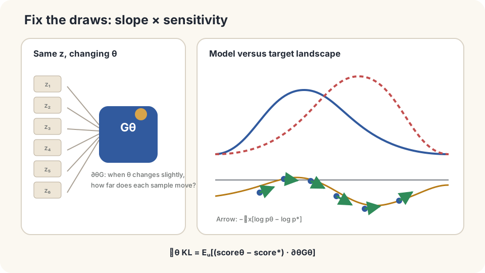
Fixed noise exposes sample motion; generator derivatives convert spatial scores into parameter updates.

Derive it in one dimension

First use scalar samples and parameters. Assume differentiable $G_\theta$, suitable smooth densities, finite KL, and justified exchanges of derivatives and integrals. The support must be parameter-independent or moving-boundary contributions correctly handled. Then

Differentiate inside the fixed-noise expectation. Parameters occur both through $G_\theta$ and explicitly in the model-density index:

Term $B$ differentiates the density parameter at fixed $x$, not along the generated sample path. Under the regularity assumptions its expectation is zero:

Changing the variable name from $G_\theta(z)$ to $x$ gives the first equality; differentiating normalization gives the final zero. Therefore

For $d$-dimensional samples and $m$ parameters, $J_\theta G\in\mathbb R^{d\times m}$ gives $\nabla_\theta L=\mathbb E_z[(J_\theta G)^\top(s_\theta-s^*)]$, where $s=\nabla_x\log p$. The result has parameter dimension $m$.

A spatial score $\nabla_x\log p$ points toward increasing log density. An $x$-independent normalizer disappears under this derivative, but is not thereby calculated. The generator supplies the Jacobian; model and target distributions supply the scores.

What information does the formula need?

At each generated sample, obtain three quantities:

1. Generator Jacobian: available through differentiation of the program.
2. Target spatial score: analytic if the target density is known; target samples alone do not directly supply it. Score estimation is another learning problem [5].
3. Model spatial score: knowing a generator does not generally expose its density or score. An invertible generator may permit change of variables; a general generator may require estimation or may not even induce an ambient-space density.

Two scores do not necessarily require two additional neural networks: analytic expressions and other estimators may exist. Bypassing normalizers in spatial derivatives does not evaluate likelihoods or KL values.

Check differentiable sample paths, score accuracy at generated locations, and the KL direction. Discrete outputs need other estimators or relaxations. Reverse KL can tolerate missing target modes, so a mode-coverage goal may call for a different discrepancy.

A Gaussian calculation with and without the extra term

Let $G_\theta(z)=\theta+z$, $z\sim\mathcal N(0,1)$, and $p^*=\mathcal N(5,1)$. KL is $(\theta-5)^2/2$. Spatial scores are $-(x-\theta)$ and $-(x-5)$, whose difference is exactly $\theta-5$ for every sample. Generator sensitivity is one, so $A$ has no sampling variation here.

import numpy as np
rng = np.random.default_rng(0)
theta, target, lr = 0., 5., .1
for step in range(60):
    z = rng.standard_normal(256)
    x = theta+z
    score_model = -(x-theta)
    score_target = -(x-target)
    grad_A = np.mean(score_model-score_target)
    grad_B = np.mean(x-theta)  # Parameter derivative at fixed x; mean zero.
    theta -= lr*grad_A
    if step%15==0:
        print(step,theta,grad_A,grad_B)
print(theta)

The update approaches five. Each batch’s $A$ equals the exact gradient, while $B$ fluctuates with mean zero. Including $B$ would add noise in this example; that observation does not establish a universal variance comparison.

Estimated scores can be inaccurate in sparse tails. Nonlinearity alone does not imply no analytic density: $\theta+|z|$ has a shifted half-normal law, but its moving support invalidates the simple zero-mean proof without boundary treatment. A low-dimensional latent mapped into higher dimensions can induce a singular law, making the displayed density-based KL undefined or infinite.

Switch generators and target information to inspect how score differences move parameters.

Check your understanding

References

1. Kingma, D. P., Welling, M. Auto-Encoding Variational Bayes. ICLR 2014.
2. Rezende, D. J., Mohamed, S., Wierstra, D. Stochastic Backpropagation and Approximate Inference in Deep Generative Models. ICML 2014.
3. Mohamed, S., Rosca, M., Figurnov, M., Mnih, A. Monte Carlo Gradient Estimation in Machine Learning. JMLR 21, 2020.
4. Roeder, G., Wu, Y., Duvenaud, D. Sticking the Landing: Simple, Lower-Variance Gradient Estimators for Variational Inference. NeurIPS 2017.
5. Hyvärinen, A. Estimation of Non-Normalized Statistical Models by Score Matching. JMLR 6, 2005.