
L0.1 One Degree or Ten: A Loss Function Declares What Matters
Builds on2 notes
Ten times worse or a hundred times worse?
A forecast of 25 degrees is slightly wrong when the temperature is 26, and badly wrong when it is 35.
How much worse is the larger error?
Squared loss makes a tenfold error a hundred times as costly; absolute loss makes it ten times as costly. A decision about clothing might instead depend on crossing a threshold. Turning accuracy into a training objective requires deciding which consequences matter.
Data alone cannot tell us how painful a ten-degree error is. The loss declares a preference supplied by the forecast’s users.
Once declared, that preference determines an ideal target. Which Temperature Should We Forecast? MSE Selects the Conditional Mean showed that squared loss selects a conditional mean and absolute loss a median. Here we examine the resulting target, outlier sensitivity, and optimization behavior.
Choosing a loss chooses the statistic to learn.
Is a ten-degree error ten or a hundred times worse?
Does the data determine that ratio,
or do the prediction’s users choose it?
DiscussionQ1
What kind of object is a loss? What changes when we replace it, and what might we sacrifice for easier optimization?
Show the reasoning
A loss assigns a penalty to a prediction and outcome. Their types can differ: a binary label is zero or one, while the prediction can be a probability.
For each input , the ideal answer is
This minimizes expected penalty within the conditional distribution at . Changing the loss can therefore change the target function itself: squared loss elicits the mean, absolute loss a median, and cross-entropy the conditional probability distribution.
Changing a loss for computational convenience may change the target. Conversely, two losses can share an unrestricted ideal target yet optimize differently. Squared probability loss and cross-entropy both elicit probabilities, but sigmoid saturation can suppress the former’s gradient when confidently wrong. Ask separately: Is this the right target, and can we train toward it?
The shape of the penalty
Plot the penalty against residual :
- Squared loss : marginal penalty grows with error. Extreme observations can pull a fitted curve strongly.
- Absolute loss : marginal penalty has constant magnitude, limiting an extreme residual’s influence.
- Huber loss: quadratic near zero and linear beyond , retaining smooth local behavior while limiting the influence of large residuals.
Cross-entropy penalizes assigning probability to the realized class by about , and by about . Confident mistakes have unbounded penalty. Binary squared probability loss is bounded by one.
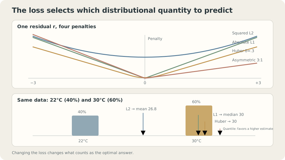
The same conditional distribution yields a mean, median, or other quantile depending on the penalty.
Where does the best answer move?
Fix and minimize conditional expected loss:
| Loss | Ideal answer | Reason |
|---|---|---|
| See M1.2 | ||
| Conditional median | ||
| Conditional -quantile | ||
| Expected loss is entropy plus KL; see M5.1 | ||
| Conditional mode | Choose the most probable class |
For cross-entropy, first allow any candidate probability distribution and expand the expected penalty:
Minimizing cross-entropy minimizes KL from the true conditional distribution. A score uniquely minimized by the truth is strictly proper. Squared probability loss, the Brier score, is also strictly proper; classification accuracy is not, because it ignores probability values beyond the winning class. This matters when probabilities inform decisions and expected costs.
DetailsProper does not mean easy to optimize
For sigmoid output , differentiate with respect to logit :
When but , the cross-entropy gradient is near . Squared loss contains the extra factor , weakening correction precisely when the prediction is confidently wrong.
Their unrestricted probability targets coincide, but their optimization landscapes differ. The example below compares recovery after 400 steps from a deliberately poor initialization.
Forecasts, property prices, and the MSE default
Forecasts: first specify which side of temperature error costs more. If overestimation is more costly, pinball loss with targets a lower quantile. The cost interpretation must match the residual’s sign.
Property prices: if underestimation costs three times as much as overestimation, pinball loss with targets the conditional 75th percentile.
When is MSE appropriate? When the conditional mean is desired, second moments exist, and squared costs match the use. It can also estimate classification probabilities, though sigmoid saturation can slow optimization.
These conclusions assume the loss represents the actual preference, extreme observations are unwanted contamination rather than important signals, and the ideal target exists and is representable. Otherwise the table describes an ideal objective rather than the fitted model’s guaranteed result.
Same data, different losses
Outliers. Add to three of thirty toy responses. Fit cubic polynomials under different losses and compare squared distance to the true conditional mean:
import numpy as np
from scipy.optimize import minimize
from ml_toy import toy_1d, truth
x, y = toy_1d()
y = y.copy()
y[[5, 14, 23]] += 2.5
xs, ys = truth()
V = np.vander(x, 4, increasing=True)
Vs = np.vander(xs, 4, increasing=True)
def fit(rho):
    w0 = np.linalg.lstsq(V, y, rcond=None)[0]
    return minimize(lambda w: rho(V @ w-y).mean(), w0, method='Powell',
                    options=dict(xtol=1e-10, ftol=1e-12, maxfev=200000)).x
losses = {
    'MSE': lambda r: r**2,
    'MAE': lambda r: np.abs(r),
    'Huber delta=0.3': lambda r: np.where(np.abs(r)<=.3, .5*r**2, .3*(np.abs(r)-.15)),
}
for name, rho in losses.items():
    w = fit(rho)
    print(name, 'squared distance to truth:', ((Vs@w-ys)**2).mean())
MSE squared distance to truth: 0.1005
MAE squared distance to truth: 0.0183
Huber delta=0.3 squared distance to truth: 0.0148Only the loss changes, yet the fitted curve’s error differs substantially. Squaring gives large residuals disproportionate influence. Huber retains quadratic behavior for small residuals and reduces that influence for large ones; its advantage here is an example, not universal dominance.
Correct target, difficult training. Fit the same linear logistic model to the two-moons toy, using the same learning rate and 400 updates, from two initializations:
import numpy as np
from ml_toy import toy_2d
X, y = toy_2d()
A = np.c_[np.ones(len(X)), X]
sig = lambda z: 1/(1+np.exp(-z))
def train(kind, w0, steps=400, lr=0.5):
    w = np.array(w0, float)
    for _ in range(steps):
        p = sig(A@w)
        g = A.T@(p-y)/len(y) if kind=='ce' else A.T@((p-y)*p*(1-p))/len(y)
        w -= lr*g
    p = sig(A@w)
    nll = -(y*np.log(p+1e-12)+(1-y)*np.log(1-p+1e-12)).mean()
    return ((p>.5)==y).mean(), nll
for w0, tag in (([0,0,0], 'zero start'), ([0,-8,8], 'confidently wrong start')):
    for kind in ('ce', 'sq'):
        acc, nll = train(kind, w0)
        print(tag, kind, 'accuracy', acc, 'NLL', nll)
# sq uses half squared loss, accounting for its omitted factor of two.
zero start cross-entropy accuracy 0.890 NLL 0.2603
zero start squared loss accuracy 0.865 NLL 0.2946
confidently wrong start cross-entropy accuracy 0.890 NLL 0.2610
confidently wrong start squared loss accuracy 0.180 NLL 9.0023From zero, both train reasonably. From the saturated wrong start, cross-entropy recovers while squared loss moves slowly because of the extra sigmoid factor. This illustrates an optimization difficulty, not a claim that squared loss is never usable for classification.
Poor initialization, an oversized update, or a previously trained model facing distribution shift can all produce confident mistakes.
A proper score locates the desired ideal minimum; it does not guarantee reaching it.
Change both the target and the gradient
Switch losses to see how the same observations produce different best predictions.
Check your understanding
References
- Gneiting, T., Raftery, A. E. Strictly Proper Scoring Rules, Prediction, and Estimation. JASA 2007.
- Huber, P. J., Ronchetti, E. M. Robust Statistics, 2nd ed. Wiley 2009, Ch. 1, 7.
- Bishop, C. M. Pattern Recognition and Machine Learning. Springer 2006, Ch. 1.5.5, 4.3.2.