U1.0 What Is a Generative Model Learning?

Builds on5 notes

A request that sounds simple

We have 50,000 32×32 images. We already know a familiar recipe from machine learning: define a loss and reduce it with gradient descent. Now someone asks for something different: can these tools produce an image the model has never seen, yet looks as though it belongs to the same dataset?

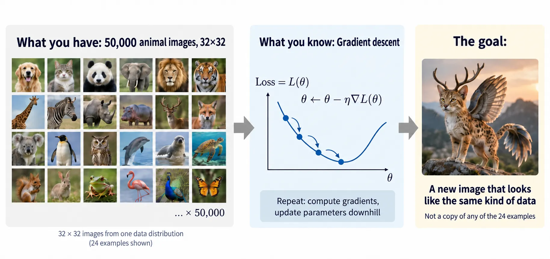
50,000 animal images, a loss curve and gradient update, and a new image marked with a question mark.

Figure: the problem we face. We have samples and know how to optimize a loss. What we want at the end is a new, plausible sample.

We will turn this intuitive request into a mathematical problem that we can implement. First we need to ask:

What does it mean to generate an image?
And what does it mean to look as though it came from the same dataset?

Generating an image from the same source

A 32×32 RGB image contains $32\times32\times3=3072$ numbers. Treat each number as a coordinate: an image is one point in $\mathbb R^{3072}$ .

SupplementWhat is a point in 3072 dimensions?

A vector containing 3072 numbers. In the more familiar $\mathbb R^3$ , a point is three numbers, such as $(1,2,-0.5)$ . We simply replace three coordinates with 3072.

Every possible image corresponds to a point in this space. Real images are not spread uniformly through it: some are common, others rare, and many points represent noise or implausible images.

A distribution describes which regions are more or less likely to contain data. We call this real but unknown distribution $p_{\text{data}}$ .

In a continuous model, $p_{\text{data}}(x)$ is a probability density: how densely data occurs near $x$ , rather than the probability of exactly $x$ . Higher density means nearby images are more common when we sample from this source.

SupplementWhy density rather than probability?

For a continuous density, a single point has probability zero, and a density value may exceed one. Multiplying by a small volume gives $p_{\text{data}}(x)\,\mathrm dx$ , approximately the probability of landing in that small region. Integrating over the whole space gives one.

Thus $p_{\text{data}}$ is a function over the entire space. If density were height, common regions would form hills and rare regions valleys. A local density peak is a mode.

Our 50,000 images are not the distribution itself; they are samples from it, or observed points in $\mathbb R^{3072}$ . They usually reveal some structure: many samples in some regions, few in others, and none in large parts of the space.

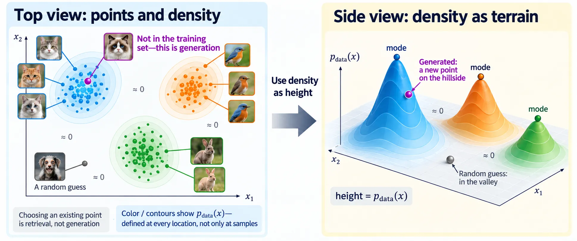
A point cloud grouped into cats, birds, and rabbits, with density contours; the same density shown as a landscape with three modes.

Figure: from samples to a distribution. The left panel shows similar images clustered together. Density has a value at every location, including locations without an observed sample. The right panel uses density as height, with modes at the peaks. This low-dimensional picture illustrates data that actually lives in $\mathbb R^{3072}$ .

We can now explain generation and resemblance together.

Generation means drawing a new point from $p_{\text{data}}$ . Selecting one of the existing images would be retrieval; we want a previously unseen sample.

Why should it resemble the dataset? It comes from the same distribution. High-density regions are sampled more often, so most samples fall in plausible regions.

There is no rule that forbids a sample from entering a low-density region. It is simply less likely to do so.

More precisely, resembling the original data means:

The new point also looks like a draw from the same $p_{\text{data}}$ .

Here is the difficulty: we cannot observe the distribution that generates the data. We see 50,000 points, but want to learn the landscape behind them.

Could a neural network represent the density directly?

A natural approach is to represent $p_\theta(x)$ with a network, fit it to $p_{\text{data}}$ , and then sample from it.

Before choosing a loss, its output must be a valid density, satisfying both:

Nonnegativity: $p_\theta(x)\geq0$ everywhere.
Normalization: $\int p_\theta(x)\,dx=1$ .

An ordinary network can output any real number, so neither condition holds automatically. We need to enforce each mathematically.

Let the network output $E_\theta(x)$ and exponentiate its negative:

\tilde p_\theta(x)=e^{-E_\theta(x)}>0.

This enforces positivity. Lower energy gives higher unnormalized density, but the total need not be one. Compute the total $Z_\theta$ and divide by it:

Z_\theta=\int \tilde p_\theta(x)\,dx, \qquad p_\theta(x)=\frac{\tilde p_\theta(x)}{Z_\theta}.

Provided $Z_\theta$ is finite, this enforces normalization. A model that assigns energies and converts them into a distribution this way is an energy-based model [1].

SupplementWhy call it energy?

The name comes from statistical physics, where the probability of a state often takes the form

p(x)\propto e^{-E(x)}.

Lower $E(x)$ makes $e^{-E(x)}$ larger and the state more likely. An energy-based model uses the same mathematical form, assigning lower energy to states it considers more plausible.

This need not be physical energy. It is a numerical measure of compatibility with the data; exponentiation and normalization still turn it into a density.

With a density in hand, we can maximize likelihood, assigning higher density where data occurs. Expanding the negative log-likelihood gives

\mathcal L_{\text{density}}(\theta) =-\mathbb E_{x\sim p_{\text{data}}}\log p_\theta(x) =\mathbb E_{x\sim p_{\text{data}}}E_\theta(x)+\log Z_\theta .

The first term lowers energy near training data. The second is difficult: $Z_\theta$ integrates over the full 3072-dimensional space and cannot be computed from our images alone.

Training actually needs the gradient rather than the value of $Z_\theta$ . Differentiating gives

\nabla_\theta\mathcal L_{\text{density}} = \mathbb E_{x\sim p_{\text{data}}}\!\left[\nabla_\theta E_\theta(x)\right] - \mathbb E_{x'\sim p_\theta}\!\left[\nabla_\theta E_\theta(x')\right].

We can estimate the first expectation using training data. The second averages over the model’s own distribution, requiring draws $x'$ from the current $p_\theta$ . We wanted to train a distribution we could sample from, yet its training gradient already requires model samples.

An expression that we can write but cannot compute directly is often called intractable. Energy-based models can be trained with approximate sampling; the issue is that direct density learning couples normalization to sampling.

Could we learn a function that produces samples instead?

Do we already know a distribution we can sample from? Yes: the standard Gaussian $\mathcal N(0,I)$ .

NotationWhy is Gaussian sampling easy?

$\mathcal N(0,I)$ is the standard Gaussian on $\mathbb R^d$ . Established algorithms directly generate Gaussian random numbers, without training another model or taking many iterative steps through the space.

In $d$ dimensions, the coordinates are independent:

z_i\overset{\text{iid}}{\sim}\mathcal N(0,1),\qquad p_z(z)=(2\pi)^{-d/2}\exp\!\Big(-\tfrac{1}{2}\|z\|^2\Big).

A $d$ -dimensional draw is just $d$ independent one-dimensional draws. This is what torch.randn(d) does.

Gaussian samples are readily available raw material. We want images from $p_{\text{data}}$ , so the question becomes:

Can a processing machine turn Gaussian raw material into the data we want?

Write this machine as a function $G$ : draw $z\sim\mathcal N(0,I)$ and compute $x=G(z)$ . If the outputs collectively follow $p_{\text{data}}$ , we have solved the generation problem:

z\sim\mathcal N(0,I)\quad\Longrightarrow\quad G(z)\sim p_{\text{data}}.

Generation now means draw $z$ , then transform it with $G$ . The resulting transformation of a distribution is its pushforward. A function $G$ that sends one distribution to another is a transport map.

DefinitionPushforward

For a distribution $p_z$ and measurable function $G$ , the distribution of transformed samples is $G_\#p_z$ . For any measurable set $A$ ,

\big(G_\#p_z\big)(A)\;=\;p_z\big(G^{-1}(A)\big),

The chance that $G(z)$ lands in $A$ equals the chance that $z$ lies in its preimage. Equivalently, for an integrable function $f$ ,

\mathbb E_{x\sim G_\#p_z}\big[f(x)\big]=\mathbb E_{z\sim p_z}\big[f(G(z))\big].

Our goal is therefore find $G$ such that $G_\#\mathcal N(0,I)=p_{\text{data}}$ .

How do we learn $G$ ? We have real samples and generated samples; we need a loss differentiable with respect to $\theta$ .

DiscussionQ1

Why not use ordinary prediction? Draw $z$ , compute $G(z)$ , and compare it with a training image using $L_2$ :

\mathcal L(\theta)=\mathbb E_{z,\,x}\big\|G_\theta(z)-x\big\|^2 .

What happens if we train this way?

Show the reasoning

$L_2$ requires pairs, but nobody has told us which noise should produce which image. Here $z$ and $x$ are sampled independently.

We can calculate the optimum. Fix $z$ ; independence gives

\arg\min_v\mathbb E_x\|v-x\|^2=\mathbb E[x] \quad\Longrightarrow\quad G_\theta(z)\equiv\mathbb E_{x\sim p_{\text{data}}}[x]\quad\text{for all }z.

Every input produces the same mean training image: a blurry, gray result with low $L_2$ but no diversity. This is regression to the mean when a prediction has multiple possible targets.

The loss asks the wrong question. We need the distribution of $G(z)$ to match $p_{\text{data}}$ , while independent-pair $L_2$ asks whether a particular output matches a particular image. Two sets can follow the same distribution without independently drawn pairs being close. This objective therefore learns the mean.

There are two natural directions:

Use a distribution-level objective to compare the generated and real distributions.
Construct the pairing ourselves. If a noise input has an assigned endpoint, perhaps even a whole path, samplewise regression can make sense again.

Let us examine the first direction before returning to constructed pairs.

If $G_\theta$ is invertible, can we recover its density?

We need a distribution-level objective. Since $G_\theta$ produces samples, perhaps we can calculate their density and train by likelihood.

Knowing how to compute $G_\theta(z)$ does not tell us the density at $x$ . We need to recover its source $z$ and account for local stretching or compression of space.

If $G_\theta$ is invertible and sufficiently smooth, the inverse recovers $z$ and the Jacobian determinant measures volume change. Change of variables gives

\log p_\theta(x)=\log p_z\!\big(G_\theta^{-1}(x)\big)+\log\Big|\det\frac{\partial G_\theta^{-1}}{\partial x}(x)\Big| .

The first term evaluates the Gaussian density at the recovered source. The second corrects for local volume change. Models that compose invertible transformations to turn simple distributions into complex ones are normalizing flows [2, 3].

If the inverse and log-determinant are tractable, we can evaluate $p_\theta(x)$ and train by maximum likelihood:

\min_\theta\ \mathcal L(\theta)=-\,\mathbb E_{x\sim p_{\text{data}}}\big[\log p_\theta(x)\big].

SupplementWhy does maximum likelihood help?

Think of $p_\theta$ as distributing a fixed supply of betting chips over the data space. The fixed total corresponds to

\int p_\theta(x)\,dx=1 .

It can put more chips in some regions and fewer in others.

For each observed image $x^{(i)}$ , we ask how much density it assigned there. Its contribution to log-likelihood is $\log p_\theta(x^{(i)})$ .

Normalization prevents assigning high density everywhere. Mass wasted in regions without data leaves less for data-rich regions. Improving likelihood therefore encourages the model to place mass where data occurs.

For $N$ independent samples,

\frac1N\sum_{i=1}^N \log p_\theta\big(x^{(i)}\big)\;\approx\;\mathbb E_{x\sim p_{\text{data}}}\big[\log p_\theta(x)\big],

Maximum likelihood maximizes average log density at the observations.

It is a distribution-level objective because

\mathrm{KL}\big(p_{\text{data}}\,\|\,p_\theta\big)=\mathbb E_{p_{\text{data}}}\big[\log p_{\text{data}}(x)\big]-\mathbb E_{p_{\text{data}}}\big[\log p_\theta(x)\big],

The first term is independent of $\theta$ . Maximizing likelihood therefore minimizes $\mathrm{KL}(p_{\text{data}}\|p_\theta)$ , which is zero exactly when the distributions agree; see M5.1.

This supplies a distribution-level loss, but every training image requires an inverse and a Jacobian determinant. An arbitrary network has no cheap inverse, and a generic $d\times d$ determinant costs $O(d^3)$ , expensive at $d=3072$ .

Normalizing flows consequently restrict their layer structures to make both calculations tractable. Their exchange for exact likelihood is:

The transformation must be invertible, with a tractable Jacobian determinant.

The same destination can be reached in many ways

Many different maps can produce the same final distribution:

G_\#p_z=p_{\text{data}} .

Imagine moving boxes between warehouses. Success means the correct final number of boxes at every location. It does not specify which box goes where or which route it follows.

Transport is therefore underdetermined. Likelihood evaluates the final distribution without selecting a unique pairing or path; normalizing flows restrict the map to calculate that likelihood.

Interactive demo: the same endpoints, different transport. Change the pairing. The Gaussian at $t=0$ and target distribution at $t=1$ stay fixed; pointwise assignments and intermediate paths change.

Could we construct the missing pairs ourselves?

Each approach has a difficulty: direct density learning requires normalization, independent-pair regression learns a mean, and exact flow likelihood restricts the transformation.

But $L_2$ itself was not the problem; arbitrary pairing was. Regression may become useful if we construct meaningful training pairs.

Instead of guessing which image a Gaussian input should become, reverse the direction. Training provides clean data $x_0$ . A rule that gradually adds noise constructs $x_1,\ldots,x_T$ ourselves.

This resembles recording a video of boxes being scattered. We know how each frame was created. Learning to reverse it can begin with a local question: given this frame, how should we move toward the preceding one?

This noise-adding rule is the forward process. It does not automatically solve the reverse direction, but supplies noisy states we can sample and separates generation into learning problems at different noise levels.

Diffusion begins by designing a forward process that constructs training pairs from data.

How should we add noise so that any $x_t$ is easy to generate and $x_T$ approaches a familiar distribution we can sample?

Check your understanding

References

LeCun, Y., Chopra, S., Hadsell, R., Ranzato, M., Huang, F. A Tutorial on Energy-Based Learning. 2006.
Papamakarios, G., Nalisnick, E., Rezende, D. J., Mohamed, S., Lakshminarayanan, B. Normalizing Flows for Probabilistic Modeling and Inference. JMLR 2021.
Rezende, D. J., Mohamed, S. Variational Inference with Normalizing Flows. ICML 2015.