M3.2 A Thousand Leaves in a Noisy River: The Fokker–Planck Equation

Builds on4 notes

Many leaves, now with fluctuations

M2.2 evolved a cloud under deterministic transport. M3.1 added fluctuations to individual paths. We now combine those descriptions.

Release a thousand leaves beneath a bridge into a river with both current and random fluctuations. How does their distribution evolve?

Even symmetric random crossings create net flux when adjacent cells contain different numbers of leaves. A crowded cell sends more walkers to its sparse neighbor than return. What term does this add to density bookkeeping?

DiscussionQ1

What represents the cloud’s law, and how does random motion modify inflow-minus-outflow accounting?

Show the reasoning

The leaves sample $p_0$ and independently follow $dx=fdt+gdW$ . Their positions at time 60 sample $p_{60}$ . We want an equation for $p(x,t)$ .

Drift contributes $-\nabla\cdot(fp)$ . Random crossings also conserve mass, but their imbalance depends on neighboring densities. The difference between a value and its neighbors’ average is governed by second derivatives: peaks lose mass and troughs gain it.

Thus expect a drift term plus a multiple of the Laplacian $\Delta p=\nabla\cdot\nabla p$ , the sum of second spatial derivatives. We still need its coefficient.

Dye in moving water

Think of a drop of dye. Current transports and deforms it; diffusion spreads it and lowers concentration near its peak. Total dye remains constant in a closed system.

Both effects contribute at first order in elapsed time. A short-step expansion lets their leading contributions add; it does not imply that two arbitrary finite-time evolution operators commute.

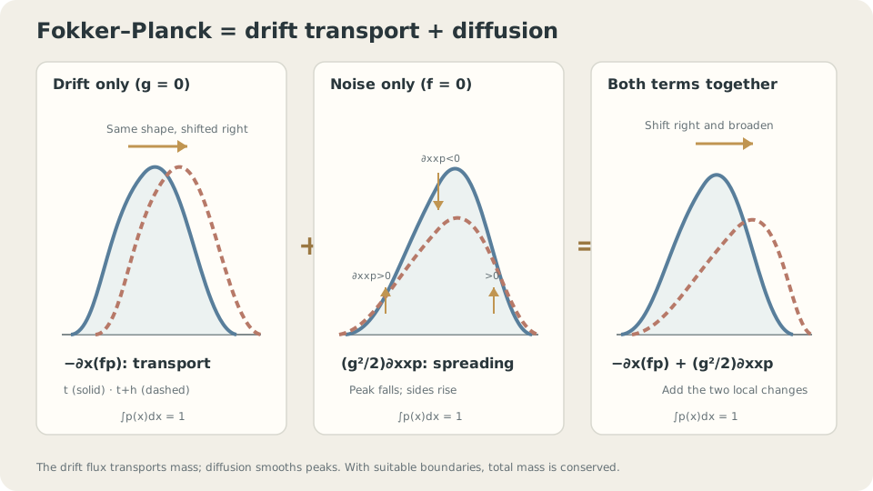
Drift transports mass while diffusion smooths density peaks and troughs.

Transport contributes first spatial derivatives; diffusion contributes second derivatives. Both conserve probability with suitable boundary behavior.

Compute the two contributions

First take one dimension with $f=0$ and constant noise intensity over a short step. Adding $g\sqrt h\varepsilon$ convolves the old density with $\mathcal N(0,g^2h)$ :

p(x,t+h)=\mathbb E_\varepsilon\big[p(x-g\sqrt h\,\varepsilon,\,t)\big].

Taylor-expand $p(x-y)$ to second order and average over standard Gaussian $\varepsilon$ . Its zero mean removes the linear term; unit variance determines the quadratic term:

p(x,t+h)=p-\,g\sqrt h\,\mathbb E[\varepsilon]\,\partial_xp+\tfrac{g^2h}{2}\,\mathbb E[\varepsilon^2]\,\partial_{xx}p+O(h^{3/2}) =p+\tfrac{g^2h}{2}\,\partial_{xx}p+O(h^{3/2}).

Subtract $p$ , divide by $h$ , and take the limit to obtain $\partial_tp=(g^2/2)\partial_{xx}p$ . The diffusion coefficient is therefore $g^2/2$ . $\square$

Drift alone gives $\partial_tp=-\partial_x(fp)$ by M2.2. Adding the two first-order time contributions gives

\boxed{\partial_tp=-\partial_x(fp)+\tfrac{g^2}{2}\partial_{xx}p},\qquad \text{in }d\text{ dimensions: }\partial_tp=-\nabla\cdot(fp)+\tfrac{g^2}{2}\Delta p.

This is the Fokker–Planck equation, also called the forward Kolmogorov equation [1–4]. It evolves the SDE’s marginal density directly, just as the continuity equation describes deterministic transport.

Verify a candidate. Solving a PDE can be difficult; substituting a proposed solution is often straightforward. For Brownian motion, $f=0$ , $g=1$ , and an origin start, test $p_t=\mathcal N(0,t)$ :

p=\frac{1}{\sqrt{2\pi t}}e^{-x^2/2t},\qquad \partial_xp=-\frac{x}{t}\,p,\qquad \partial_{xx}p=\Big(-\frac1t+\frac{x^2}{t^2}\Big)p,\qquad \partial_tp=\Big(-\frac{1}{2t}+\frac{x^2}{2t^2}\Big)p .

The right side is $\tfrac12\partial_{xx}p=(-\tfrac1{2t}+\tfrac{x^2}{2t^2})p=\partial_tp$ for $t>0$ . As $t\to0$ , this Gaussian converges weakly to $\delta_0$ , matching the initial law. The PDE alone would not specify the intended solution without initial and applicable boundary conditions.

DetailsConstant drift: verify N(ct,g²t) from an origin start

Let m=ct, s=g²t, and p=(2πs)^(−1/2)exp(−(x−m)²/(2s)). Then ∂ₓp=−(x−m)p/s and ∂ₓₓp=[−1/s+(x−m)²/s²]p. Differentiating log p with m′=c and s′=g² yields ∂ₜp=[−g²/(2s)+c(x−m)/s+g²(x−m)²/(2s²)]p. The drift term supplies c(x−m)p/s and diffusion supplies the other two terms. Their sum equals ∂ₜp.

For positive smooth density and position-independent g, (g²/2)Δp=∇·[p(g²/2)∇log p]. Thus the same density equation can be written ∂ₜp+∇·(pu)=0 with u=f−(g²/2)∇log p. Under suitable existence and uniqueness conditions, an ODE with this velocity can share the SDE’s marginal laws, while having different trajectories and temporal couplings.

What the width formula assumes

Constant drift gives variance $g^2t$ . General drift can compress or expand the cloud: in one dimension, $\frac d{dt}\operatorname{Var}(x_t)=2\operatorname{Cov}(x_t,f(x_t,t))+g(t)^2$ , under suitable integrability. Diffusion smooths locally without guaranteeing a unimodal combined distribution.

A restoring drift can balance diffusion and produce equilibrium. That is the next note’s question, M3.3.

Here $g(t)$ is a scalar independent of position, with independent equal-intensity Brownian coordinates. State-dependent Itô diffusion instead contributes $\tfrac12\partial_{xx}(g^2p)$ in one dimension. Non-Gaussian iid small steps can share a diffusion limit under appropriate conditions; their finite-step increments are still not Brownian increments.

Compare a histogram and change the noise

import numpy as np
rng = np.random.default_rng(0)
c, g, T, h = .5, .3, 60., .1
x = np.zeros(20000)
for _ in range(int(T/h)):
    x += h*c+g*np.sqrt(h)*rng.standard_normal(x.size)
hist, edges = np.histogram(x,bins=60,density=True)
mid = .5*(edges[1:]+edges[:-1])
p_theory = np.exp(-(mid-c*T)**2/(2*g**2*T))/np.sqrt(2*np.pi*g**2*T)
print(np.abs(hist-p_theory).max())
# Try Cauchy increments: their infinite variance invalidates this derivation.

Compare against $\mathcal N(cT,g^2T)$ . Cauchy increments require a different scaling and evolution equation; repeated $\sqrt h$ -scaled Cauchy steps do not converge to this fixed-scale Brownian model.

Equal-variance uniform increments agree with Gaussian increments in an appropriate diffusion limit. At finite step size, their increment distributions still differ.

Check your understanding

References

Särkkä, S., Solin, A. Applied Stochastic Differential Equations. Cambridge University Press, 2019.
Pavliotis, G. A. Stochastic Processes and Applications: Diffusion Processes, the Fokker–Planck and Langevin Equations. Springer, 2014.
Risken, H. The Fokker–Planck Equation: Methods of Solution and Applications. Springer, 2nd ed., 1989.
Gardiner, C. Stochastic Methods: A Handbook for the Natural and Social Sciences. Springer, 4th ed., 2009.