M2.2 Change in the Crowd = Inflow − Outflow: The Continuity Equation

Builds on3 notes

Back to the station

M0.1 counted net flow through a station’s gates. Integrating divergence gives the total outward flux.

Now consider the entire concourse: people walk toward platforms, exits, or ticket machines. Suppose we know their velocity at every position and time, together with the current crowd density. Where will the crowd concentrate ten minutes later?

M2.1 followed every person and transported the distribution. Alternatively, watch a fixed floor tile: how much enters and leaves? Can these local counts describe density evolution directly?

DiscussionQ1

Apply “change = inflow − outflow” to one square floor tile. Which quantities determine the crossings?

Show the reasoning

Count people crossing its edges, then express those counts using density and velocity.

The number on a tile is approximately density times area. Across an edge, the crossing rate is density times the normal velocity component times edge length. The vector flux is $pv$ , mass per unit boundary length per unit time in two dimensions.

Net horizontal inflow is $(pu_1)_{\mathrm{left}}-(pu_1)_{\mathrm{right}}$ , times edge length; similarly vertically. For a small tile, these differences give net inflow

\begin{aligned} &-[\partial_x(pu_1)+\partial_y(pu_2)]\,\Delta A\\ &\qquad=-\nabla\cdot(pu)\,\Delta A. \end{aligned}

Thus the tile’s density changes at minus the divergence of its flux. If a randomly chosen person’s position is the random variable, $p(x,t)$ is the density we want to evolve.

A bookkeeper on every tile

Imagine a bookkeeper on each tile, recording crossings without knowing anyone’s origin or destination.

Their local accounts jointly describe the distribution. This replaces the Lagrangian view, following particles, with the Eulerian view, observing fixed locations. The previous flow map and the continuity equation describe the same transport from these two viewpoints.

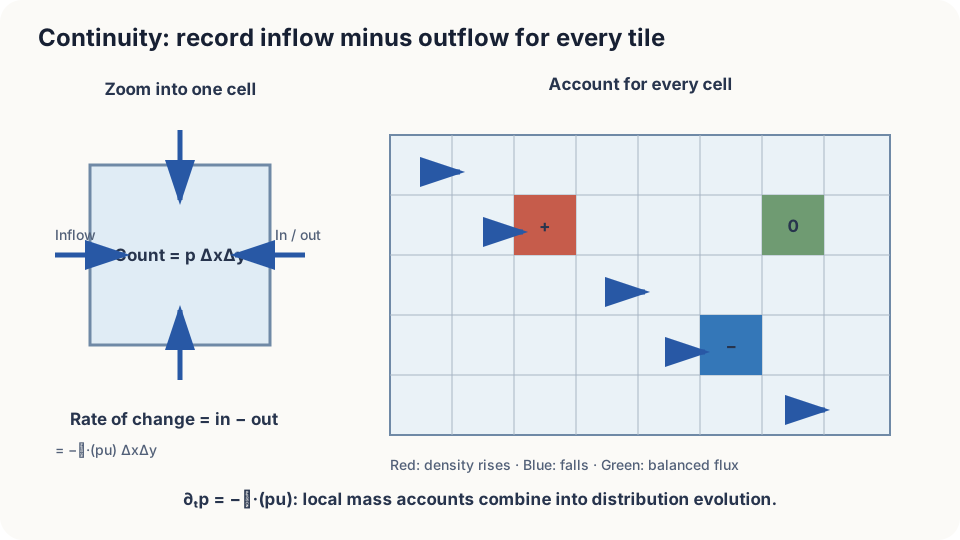
Boundary flux on one tile and mass accounting across the whole grid.

Local density changes equal inflow minus outflow; all local accounts together evolve the distribution.

Derive it on one box

Let $p$ be density, $v$ velocity, and $J=pv$ flux. A fixed region $B$ contains mass $\int_B p\,dx$ . With no internal sources or sinks, its mass can change only through boundary crossings:

\frac{d}{dt}\int_B p\,dx\;=\;-\oint_{\partial B} p\,v\cdot n\,dS\;=\;-\int_B \nabla\cdot(pv)\,dx .

The first equality expresses conservation: the normal $n$ points outward, hence the minus sign. The second uses the divergence theorem. Since $B$ is fixed, differentiating under the integral gives $\int_B\partial_t p\,dx$ , provided the required regularity holds. Thus every region $B$ satisfies

\int_B\Big[\partial_t p+\nabla\cdot(pv)\Big]dx=0 .

A continuous function whose integral vanishes on every small region is zero everywhere. Therefore

\boxed{\;\partial_t p+\nabla\cdot(p\,v)=0\;}

This is the continuity equation: density changes at minus the flux divergence. Outward spreading lowers density; inward convergence raises it. $\square$

This is a partial differential equation in space and time. Initial density, velocity, and appropriate boundary conditions define an evolution problem; obtaining its solution may still require numerical approximation.

Connection to pushforwards. Under suitable Lipschitz and existence assumptions, the solution is $(\Phi_t)_\#p_0$ [3, Chapter 8]. For $\dot x=-x$ and $p_0=\mathcal N(0,1)$ , the earlier result $p_t=\mathcal N(0,e^{-2t})$ satisfies $\partial_t p+\partial_x(-xp)=0$ directly.

DetailsCheck a Gaussian with variance σ²=e^(−2t) and velocity −x

Write p=(2πσ²)^(−1/2)exp(−x²/(2σ²)). Then ∂ₓp=−(x/σ²)p, so ∂ₓ(−xp)=(−1+x²/σ²)p. Also log p=−½log(2πσ²)−x²/(2σ²), hence ∂ₜlog p=−½(σ²)′/σ²+(x²/2)(σ²)′/σ⁴. Substituting (σ²)′=−2σ² gives ∂ₜp=(1−x²/σ²)p. The two contributions cancel exactly.

Along a trajectory, $\frac{d}{dt}p(x_t,t)=\partial_t p+v\cdot\nabla p$ . Expanding $\nabla\cdot(pv)=v\cdot\nabla p+p\nabla\cdot v$ and dividing by positive density gives

\frac{d}{dt}\log p(x_t,t)=-\nabla\cdot v(x_t,t).

Following a particle, local expansion lowers the density around it. This is the differential form of the flow-map change-of-variables formula.

What conservation does and does not determine

The pointwise derivation assumes sufficient smoothness and valid exchanges of derivatives and integrals. Integral or weak formulations extend conservation to less regular settings. In an open station, total mass inside also depends on the boundary flux.

A density path $p_t$ does not uniquely determine velocity. If $v$ satisfies the equation and $\nabla\cdot(pw)=0$ , then $v+w$ does too:

\partial_t p+\nabla\cdot\big(p(v+w)\big)=\underbrace{\partial_t p+\nabla\cdot(pu)}_{=0}+\underbrace{\nabla\cdot(pw)}_{=0}=0 .

For a rotationally symmetric Gaussian, $w(x,y)=(-y,x)$ has both $w\cdot\nabla p=0$ and $\nabla\cdot w=0$ , so $\nabla\cdot(pw)=0$ . Moving along level sets alone would not establish the flux condition. Different trajectories can therefore share the same marginal distributions.

Compute it, then test its limits

A conservative upwind discretization approximates $\partial_t p+\partial_x(pu)=0$ . For $v=-x$ and a standard Gaussian start, compare against the exact Gaussian:

import numpy as np
x = np.linspace(-4, 4, 801)
dx = x[1] - x[0]
dt = 0.002
p = np.exp(-x**2 / 2) / np.sqrt(2 * np.pi)
u_face = -(x[:-1] + x[1:]) / 2
for _ in range(int(1.0 / dt)):
    flux = np.zeros(len(p) + 1)  # Zero boundary flux on the truncated domain
    flux[1:-1] = np.where(u_face >= 0, u_face * p[:-1], u_face * p[1:])
    p -= dt * np.diff(flux) / dx
s2 = np.exp(-2.0)
exact = np.exp(-x**2 / (2*s2)) / np.sqrt(2*np.pi*s2)
print(np.abs(p - exact).max())

The finite domain introduces a small truncation error; the example imposes zero boundary flux. Refining space also requires a stable time step, here $\max|u|\,dt/dx\le1$ . With discontinuous $v=\operatorname{sign}(x)$ , outward motion leaves a central gap. Ordinary derivatives fail at the discontinuity, requiring a weak formulation and a conservative numerical treatment.

Check your understanding

References

Evans, L. C. Partial Differential Equations. AMS Graduate Studies in Mathematics 19, 2nd ed., 2010.
Villani, C. Topics in Optimal Transportation. AMS Graduate Studies in Mathematics 58, 2003.
Ambrosio, L., Gigli, N., Savaré, G. Gradient Flows in Metric Spaces and in the Space of Probability Measures. Birkhäuser, 2nd ed., 2008..）