M0.2 Thirty Seconds Without GPS: Taylor Expansion and Straight-Line Prediction

Between location updates

A navigation display receives positions intermittently. Between updates it may extrapolate using the last position and velocity.

Suppose a car travels at 10 m/s around a bend of radius 20 m, immediately after its last location update.

Prediction misses the changing velocity direction. Can current velocity and its rate of change estimate that error?

DiscussionQ1

What function is being approximated, what does straight-line prediction compute, and what error do we want?

Show the reasoning

Specify a time-dependent position rather than merely a road shape.

The vector function $x(t)$ maps time to planar position. We know its current position and velocity.

The predicted future position is

\tilde x(t+h)=x(t)+h\,\dot x(t)

This replaces the trajectory by its tangent line in time.

We seek the distance between this prediction and the actual future position. Taylor expansion quantifies how long this local approximation remains accurate.

A curved ruler looks straight up close

A short segment of a curved ruler appears straight; a longer segment reveals its deviation.

For a time-parametrized position, acceleration controls departure from constant-velocity prediction. It includes changing speed along a straight route. When a nonzero quadratic term dominates, doubling a small interval approximately quadruples error.

The observed interval plays the role of the short ruler segment.

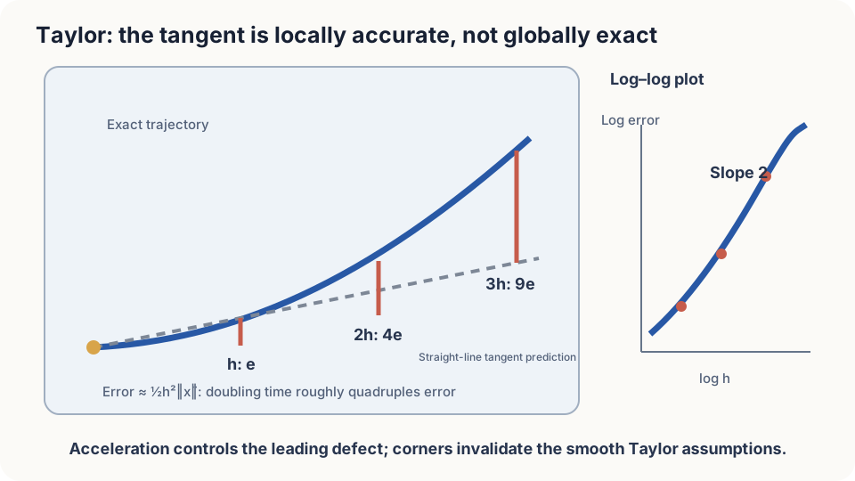
A smooth curve departs from its tangent with leading quadratic error.

Figure: tangent approximation has a leading $h^2$ remainder under suitable smoothness.

Calculate the error of constant-velocity prediction

For one scalar coordinate with suitable second differentiability,

\begin{aligned} f(t+h)&=f(t)+hf'(t)+R_1(h),\\ R_1(h)&=\frac{h^2}{2}f''(\xi),\qquad \xi\in[t,t+h]. \end{aligned}

If $|f''|\leq M$ on the interval, the remainder is at most $Mh^2/2$ . Doubling $h$ quadruples this bound for the same $M$ ; actual errors also depend on variation of the second derivative.

DetailsDerive the integral remainder

Apply the fundamental theorem twice: $f(t+h)-f(t)=\int_t^{t+h}f'(s)ds$ and $f'(s)=f'(t)+\int_t^sf''(r)dr$ . Exchange integration order:

f(t+h)-f(t)-h f'(t)=\int_t^{t+h}\!\!\int_t^{s}f''(r)\,dr\,ds=\int_t^{t+h}(t+h-r)\,f''(r)\,dr .

The weight integrates to $h^2/2$ , giving the norm bound. Continuity yields the scalar intermediate-point form; vector trajectories can use the integral bound directly without assuming one common intermediate point for every component.

Second-order Taylor includes current acceleration:

f(t+h)=f(t)+h f'(t)+\frac{h^2}{2}f''(t)+R_2(h),\qquad |R_2(h)|\le\frac{h^3}{6}\max|f'''| .

An additional derivative supports one more power of step size in the remainder, provided the required derivatives are bounded. A useful leading approximation needs an interval small enough for those derivatives to vary moderately.

Three intervals

For uniform circular motion with radius 20 m and speed 10 m/s, acceleration magnitude is $v^2/R=5$ m/s². Hence

\|x(t+h)-\widetilde x(t+h)\|\leq\frac{h^2v^2}{2R}=2.5h^2\ \text{m}.

At one second, the bound is 2.5 m and actual error about 2.48 m. At two seconds, they are 10 m and about 9.73 m, close to quadratic scaling.

At thirty seconds, the 2250 m bound remains valid but loose: actual error is roughly 290 m. The car circles within a bounded area while its tangent prediction travels 300 m away. The local quadratic approximation no longer describes the actual error well over that interval.

A bounded acceleration gives a rigorous upper bound. A nearly unchanged acceleration over a short step gives a useful leading term. Constant-speed straight motion alone makes this error zero; straight motion with changing speed does not.

Adding acceleration improves the one-second example to a cubic remainder bound near 0.42 m. M2.4 asks whether multiple velocity queries can supply this correction without directly measuring acceleration.

Run the example and tighten the turn

import numpy as np
def err(h, v=10.0, R=20.0):
    th = v*h/R
    true = R*np.array([np.sin(th), 1-np.cos(th)])
    pred = np.array([v*h, 0.0])
    return np.linalg.norm(true-pred)
hs = np.array([0.125, 0.25, 0.5, 1, 2, 4])
for R in (20.0, 2.0):
    e = np.array([err(h, R=R) for h in hs])
    print(f"R={R}: errors {np.round(e, 2)}")
    print("ratios", np.round(e[1:]/e[:-1], 2),
          "bounds", np.round(50*hs**2/R, 2))

For the wider turn, small-step ratios are close to four. The tight turn leaves that regime earlier because velocity changes faster within the same interval.

A nonsmooth corner can invalidate Taylor’s assumptions entirely. After an instantaneous direction change, constant-velocity prediction may accumulate error linearly in the remaining interval rather than quadratically.

Check your understanding

References

Strang, G. Calculus. Wellesley-Cambridge Press; MIT OpenCourseWare RES.18-001
Hairer, E., Nørsett, S. P., Wanner, G. Solving Ordinary Differential Equations I: Nonstiff Problems, 2nd ed. Springer 1993.