M3.1 Flow Plus Fluctuations: Stochastic Differential Equations

Builds on2 notes

The same river, now with fluctuations

Return to the river in M2.0. A steady current carries a leaf downstream at 0.5 m/s, while small random fluctuations push it unpredictably.

Where is a leaf released beneath the bridge one minute later?

Drift moves it downstream, but identical starting points can now yield different paths. How can one rule combine these motions? Drift displacement scales as $h$ , while Brownian perturbations scale as $\sqrt h$ .

DiscussionQ1

What represents the current and the fluctuations? Is the position after a minute a number or a random variable? How should we modify the ODE?

Show the reasoning

Writing ordinary velocity plus noise is misleading: Brownian paths are not ordinarily differentiable. Use increments instead.

Over a short interval, the ODE gives displacement approximately $f(x,t)h$ . Add $g$ times the independent Brownian increment $W_{t+h}-W_t\sim\mathcal N(0,h)$ :

x(t+h)-x(t)\;\approx\;f(x,t)\,h\;+\;g(t)\,\big(W_{t+h}-W_t\big).

The infinitesimal notation is

dx_t=f(x_t,t)\,dt+g(t)\,dW_t .

This is a stochastic differential equation (SDE), with drift $f$ and diffusion coefficient $g$ . Its solution is a random process. Fixing one Brownian realization gives one trajectory; $x_{60}$ is a random variable at one time, and its marginal law is not the whole process.

A trajectory becomes a fan

For constant $f=c$ and $g$ , paths spread around $x_0+ct$ with standard deviation $g\sqrt t$ . This is a special case: a restoring drift can prevent variance from increasing indefinitely.

Generally the solution is not an ODE solution plus Brownian motion. Random displacement changes the drift subsequently encountered. Under appropriate integrability, $\frac{d}{dt}\mathbb E[x_t]=\mathbb E[f(x_t,t)]$ , generally different from $f(\mathbb E[x_t],t)$ .

A single deterministic path becomes a fan of stochastic paths.

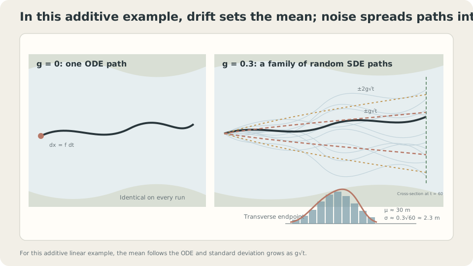
For constant drift and diffusion, the center translates and the standard deviation grows as $g\sqrt t$ .

Read the increments and simulate them

Under appropriate existence, uniqueness, and convergence assumptions, a small step admits the approximation

x_{t+h}\approx x_t+f(x_t,t)h+g(t)\sqrt h\varepsilon_t,\qquad \varepsilon_t\sim\mathcal N(0,I)\text{ independently}.

This Euler–Maruyama approximation is not an exact finite-step equality. The Itô equation is defined by $x_t=x_0+\int_0^t f(x_s,s)ds+\int_0^t g(s)dW_s$ [1,3]. We first interpret its increments; convergence comes later.

Euler–Maruyama. Turn the approximation into an update:

x_{n+1}=x_n+h\,f(x_n,t_n)+g(t_n)\sqrt h\,\varepsilon_n .

It adds noise to Euler’s method from M2.3 and reduces to Euler when $g\equiv0$ .

Check the scale. For constant $g$ , $N=T/h$ independent noise increments sum to $\sum_n g\sqrt h\varepsilon_n$ . Their variances add:

\mathrm{Var}\Big(\sum_{n=0}^{N-1}g\sqrt h\,\varepsilon_n\Big)=N\,g^2h=g^2T .

The total is independent of $h$ . Replacing $\sqrt h$ with $h$ gives variance $g^2hT\to0$ , converging to a different, noiseless model rather than approximating the intended Brownian perturbation. $\square$

An exact check. For constant $f=c$ and $g$ , summing the increments gives $x_T=x_0+cT+gW_T$ , hence

x_T\sim\mathcal N\big(x_0+cT,\;g^2T\big).

With $x_0=0$ , $c=0.5$ , $g=0.3$ , and $T=60$ , the mean is 30 m and the standard deviation is $0.3\sqrt{60}\approx2.3$ m.

DetailsWhat the increment interpretation leaves implicit

Evaluating noise intensity at each step’s start corresponds to the Itô convention. For deterministic time-dependent g, ordinary endpoint choices agree in the limit under suitable regularity. With state-dependent g(x), Itô and Stratonovich conventions differ: in one dimension their drift conversion contains ½g∂ₓg. A properly defined midpoint interpretation yields Stratonovich, rather than merely changing notation. This unit focuses on g=g(t), avoiding that distinction. Rigorous convergence also needs proof; see M3.4 and [4].

Put numbers on the uncertainty

In this example, the mean is 30 m downstream and about 95% of endpoints lie within approximately $30\pm4.6$ m. The uncertainty comes from $g\sqrt T$ , the square-root law in M3.0.

This model assumes independent Gaussian Brownian increments with variance proportional to elapsed time, and position-independent $g$ . Real eddies can have temporal correlation and spatially varying intensity. Those require a different effective model or explicit state-dependent coefficients; the size and direction of the discrepancy must be analyzed rather than assumed.

Simulate the correct and incorrect scales

import numpy as np
rng = np.random.default_rng(0)
def em(f, g, x0, T, h, trials=20000, noise_scale='sqrt'):
    x = np.full(trials, x0)
    N = int(round(T/h))
    for n in range(N):
        eps = rng.standard_normal(trials)
        step = np.sqrt(h) if noise_scale == 'sqrt' else h
        x = x + h*f(x) + g*step*eps
    return x
for h in [1.0, 0.1, 0.01]:
    ok = em(lambda x: 0.5, 0.3, 0.0, 60.0, h)
    bad = em(lambda x: 0.5, 0.3, 0.0, 60.0, h, noise_scale='h')
    print(h, round(ok.mean(),2), round(ok.std(),2), '| h-scaled std:', round(bad.std(),3))
# Correct scale: mean near 30 and standard deviation near 2.32 at every h.

Square-root scaling matches the exact Gaussian. With stationary correlated AR(1) increments and fixed $0<\rho<1$ , the discrete noise is not independent Brownian noise. A suitable limit can introduce an effective variance factor $(1+\rho)/(1-\rho)$ ; changing correlation time with $h$ requires additional analysis.

Check your understanding

References

Särkkä, S., Solin, A. Applied Stochastic Differential Equations. Cambridge University Press, 2019.
Higham, D. J. An Algorithmic Introduction to Numerical Simulation of Stochastic Differential Equations. SIAM Review 43(3), 2001.
Øksendal, B. Stochastic Differential Equations: An Introduction with Applications. Springer, 6th ed., 2003.
Kloeden, P. E., Platen, E. Numerical Solution of Stochastic Differential Equations. Springer, 1992.