M3.4 Matching Paths or Matching Statistics: Strong and Weak Convergence

A hundred simulated price paths

You simulate a stock-price SDE using daily Euler–Maruyama updates for one year. Someone asks whether the simulation is accurate.

A hundred plausible-looking curves do not settle that question. Two different requirements are possible:

1. Match corresponding paths: under a specified Brownian realization, the approximation should remain close to the exact solution driven by that same realization.
2. Match terminal statistics: means, variances, or event probabilities should be close, without requiring individual paths to match.

Like comparing trips, we can compare matched travelers or just their endpoint distributions. Does one numerical method have the same error rate under these two comparisons? Define the measures before deciding the computational budget.

Two measuring sticks

Imagine two reviewers inspecting the simulation.

One overlays every approximate path on its corresponding exact path and averages endpoint distances: the strong comparison.

The other ignores pairings and compares endpoint distributions through statistics or histograms: the weak viewpoint. A histogram is an illustration, not the formal smooth-test-function definition.

Pathwise distances retain both signs of random deviations. Taking expectations first can cancel zero-mean terms, suggesting a better weak rate in some settings. Distinct rates are not universal for all equations and statistics.

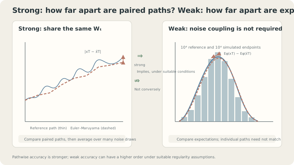
Strong error uses a shared-noise coupling; weak error compares expectations under marginal laws.

One method, two orders

ODE Euler has first-order global error. For general SDEs, Euler–Maruyama instead has the usual guarantees [1,2]:

These require appropriate Lipschitz, growth, and moment assumptions; weak order one additionally needs smoothness of coefficients and test functions. They are guarantees, not exact rates in every example. Additive noise can improve strong order, and some statistics can have zero bias.

Consider multiplicative noise $dx=\sigma x\,dW_t$. Euler–Maruyama gives $\hat x_{t+h}=\hat x_t(1+\sigma\Delta W)$. The exact Itô solution gives $x_{t+h}=x_t\exp(\sigma\Delta W-\tfrac12\sigma^2h)$. Expand:

The first omitted term is $\tfrac12\sigma^2x_t[(\Delta W)^2-h]$. Measure it in two ways:

• Strong: $(\Delta W)^2-h$ has standard deviation $\sqrt2h$. Weighted by the current state, these terms are not iid, but have conditional mean zero. Appropriate martingale second-moment and propagation estimates lead to global $O(\sqrt h)$.
• Weak: the leading omitted term has mean zero. For suitable smooth statistics, the remaining local bias is $O(h^2)$, accumulating to global $O(h)$.

The leading random defect matters pathwise but cancels at first order in the expectation calculation. The full rate proofs also control propagation and remainders.

Which comparison does the application need?

The accuracy question depends on what the simulation is used for:

• For terminal means or moments, inspect the corresponding weak bias. A rate alone does not determine whether a daily step is accurate enough, because its constant also matters.
• For approximation under a prescribed common Brownian path, inspect strong error. This mathematical coupling does not ask the simulator to predict the real world’s next random realization.

Sampling often emphasizes distributional accuracy, but matching one mean does not establish an entire law. Distances such as Wasserstein can also be useful, sometimes bounded through strong couplings. Choose the measure from the goal.

Indicator statistics require separate weak-rate analysis. Sharing noise can also reduce variance in estimates of weak differences, though shared noise is not part of the weak-error definition.

Measure the two slopes

import numpy as np
rng = np.random.default_rng(1)
sigma, T, M = 1., 1., 20000
W_fine = np.cumsum(np.sqrt(1/4096)*rng.standard_normal((M,4096)),axis=1)
x_true = np.exp(sigma*W_fine[:,-1]-.5*sigma**2*T)
for h in [1/16,1/64,1/256]:
    k = int(4096*h)
    dW = np.diff(np.concatenate([np.zeros((M,1)),W_fine[:,k-1::k]],axis=1),axis=1)
    x_em = np.prod(1+sigma*dW,axis=1)
    strong = np.abs(x_em-x_true).mean()
    weak_exact = abs((1+sigma**2*h)**(T/h)-np.exp(sigma**2*T))
    weak_mc = abs((x_em**2).mean()-np.exp(sigma**2*T))
    print(h,strong,weak_exact,weak_mc)
# The exact endpoint uses the same Brownian terminal value, not a fine Euler path.
# Strong estimates contain sampling uncertainty; weak_exact is analytic for x².

Reducing $h$ by four should roughly halve the strong error and quarter the analytic weak bias. For $\varphi=x^2$, $\mathbb E[\hat x_T^2]=(1+\sigma^2h)^{T/h}$ while the exact moment is $e^{\sigma^2T}$. Log–log slopes approach one half and one, respectively.

The empirical weak estimate may fluctuate more than its discretization bias. At these parameters, the standard deviation of $x_T^2$ is about 20, giving sampling uncertainty around $20/\sqrt{20000}\approx0.14$. More steps do not remove that Monte Carlo error.

Why not use $\varphi=x$? Here Euler–Maruyama preserves $\mathbb E[\hat x_T]=1$ exactly for every grid, so its mean has zero weak bias and cannot reveal the expected nonzero slope.

Try the indicator $\mathbb1[x>1]$, but do not assume a rate without analysis. Independently sampling the two Brownian paths also destroys the specified strong comparison: even two exact independent endpoints can be far apart.

Check your understanding

References

1. Kloeden, P. E., Platen, E. Numerical Solution of Stochastic Differential Equations. Springer, 1992.
2. Higham, D. J. An Algorithmic Introduction to Numerical Simulation of Stochastic Differential Equations. SIAM Review 43(3), 2001.
3. Särkkä, S., Solin, A. Applied Stochastic Differential Equations. Cambridge University Press, 2019.
4. Milstein, G. N., Tretyakov, M. V. Stochastic Numerics for Mathematical Physics. Springer, 2004.