M4.2 The Phone Can Ring Anytime: Continuous-Time Markov Chains

Builds on2 notes

One operator, one phone line

Calls arrive at an average of three per hour; a call lasts ten minutes on average. Calls arriving while the line is busy are rejected rather than queued.

What fraction of time is the operator busy?

Multiplying three calls by ten minutes counts rejected calls as served. Model arrivals as a Poisson process with rate $\lambda=3$ per hour and independent exponential service times with rate $\mu=6$ . These distributional assumptions do not follow from the means alone.

DiscussionQ1

What are the states? If three per hour is not a probability, how does it determine a short-time transition?

Show the reasoning

Let $X_t$ be idle (0) or busy (1), with continuous time measured in hours.

A rate is a short-time probability slope. For Poisson arrivals, one event in $\Delta t$ has probability $\lambda\Delta t+O(\Delta t^2)$ and multiple events have probability $O(\Delta t^2)$ . A rate may exceed one. The service rate $\mu$ is conditional on being busy, not the unconditional number completed each hour.

For small $\Delta t$ , transitions are approximately $\begin{pmatrix}1-\lambda\Delta t&\lambda\Delta t\\\mu\Delta t&1-\mu\Delta t\end{pmatrix}$ . This approximation can fail at large intervals. The interval-independent object is its derivative at zero: the rate matrix.

Memoryless alarms

A token in the idle square waits for an exponential alarm of rate three, then moves to busy. There it waits for an alarm of rate six, then returns. Each alarm’s remaining law does not depend on time already waited.

Rates describe short-time slopes rather than a chosen round length. They determine holding times and destinations on departure.

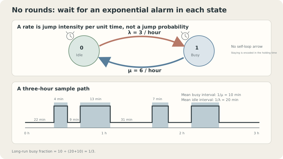
Two states with memoryless exponential alarms.

Rates determine exponential holding times; long-run occupancy reflects the mean durations of the two parts of a cycle.

Write the generator

From short-time probabilities to rates

Express the short-time matrix as

P(\Delta t)\approx I+R\,\Delta t,\qquad R=\begin{pmatrix}-\lambda&\lambda\\ \mu&-\mu\end{pmatrix}=\begin{pmatrix}-3&3\\6&-6\end{pmatrix}.

The rate matrix, or generator, has $R(x,y)\ge0$ off the diagonal and $R(x,x)=-\sum_{y\ne x}R(x,y)$ . Row sums are zero, reflecting probability conservation. Formally $R=\lim_{\Delta t\to0}[P(\Delta t)-I]/\Delta t$ .

Evolve for a finite interval

Time-homogeneous Markov transitions compose by $P(t+s)=P(t)P(s)$ . Subdivide time and take the limit:

P(t)=\lim_{n\to\infty}\Big(I+\frac{tR}{n}\Big)^{n}=e^{tR}\equiv\sum_{k\ge0}\frac{(tR)^k}{k!}.

This is the matrix analogue of the exponential limit. Differentiating also gives

\frac{d}{dt}P(t)=\lim_{\Delta t\to0}\frac{P(t)P(\Delta t)-P(t)}{\Delta t}=P(t)\,R,\qquad P(0)=I,

The resulting linear matrix ODE has solution $e^{tR}$ .

The forward equation

For row-vector initial law $p_0$ , $p_t=p_0P(t)$ satisfies

\dot p_t=p_tR\quad\Longleftrightarrow\quad \dot p_t(y)=\sum_{x\ne y}\Big[p_t(x)R(x,y)-p_t(y)R(y,x)\Big].

Expanding the diagonal term shows that each state’s change equals inflow minus outflow. This is the forward equation, also called the master equation.

It parallels M3.2 on a finite state space. Probability conservation follows from $\frac d{dt}\sum_y p_t(y)=p_tR\mathbb1=0$ .

Solve the two-state example

Busy probability satisfies $\dot p_t(1)=\lambda-(\lambda+\mu)p_t(1)$ , giving

p_t(1)=\frac{\lambda}{\lambda+\mu}+\Big(p_0(1)-\frac{\lambda}{\lambda+\mu}\Big)e^{-(\lambda+\mu)t}.

The stationary law solves $\pi R=0$ , or $\pi(0)\lambda=\pi(1)\mu$ :

\pi(1)=\frac{\lambda}{\lambda+\mu}=\frac{3}{3+6}=\frac13 .

Busy occupancy is one third, not one half. Initial-state influence decays on time scale $1/(\lambda+\mu)=1/9$ hour, about seven minutes. The nonzero generator eigenvalue supplies the exponential decay rate.

DetailsExact transitions, holding times, and oversized Euler steps

Let Π have every row equal to π. Then $R\Pi=\Pi R=0$ and $R^2=-(\lambda+\mu)R$ , so $e^{tR}=\Pi+e^{-(\lambda+\mu)t}(I-\Pi)$ . It equals I at zero, tends to Π, and has derivative R at zero.

The probability of staying in state $x$ beyond time $t$ is $e^{-|R(x,x)|t}$ . Holding times are exponential with mean $1/|R(x,x)|$ , the continuous analogue of geometric memorylessness.

The Euler approximation $I+R\Delta t$ is stochastic only if its diagonal entries stay nonnegative: here $\Delta t\le1/6$ hour. At half an hour it gives invalid probabilities. The exact matrix $e^{tR}$ remains stochastic for every $t\ge0$ .

Why the naive one-half answer fails

Only idle-line arrivals are accepted, at rate $\lambda\pi(0)=3\times2/3=2$ per hour. Two ten-minute calls occupy twenty minutes, giving one third. A queue would require different states; the offered load one half is not the occupancy of this loss system.

With Poisson arrivals and independent finite-mean nonexponential service, the renewal-cycle busy fraction remains $\mathbb E[S]/(1/\lambda+\mathbb E[S])$ . But idle/busy alone is generally no longer this CTMC, and transient probabilities and residual service times change. Time-varying arrival rates also require a time-dependent analysis.

Try it

import numpy as np
rng = np.random.default_rng(0)
lam, mu, T = 3., 6., 20000.
t, x, busy = 0., 0, 0.
while t<T:
    stay = rng.exponential(1/lam if x==0 else 1/mu)
    busy += min(stay,T-t)*x  # Truncate the final holding interval.
    t += stay
    x = 1-x
print('busy fraction:',busy/T)
# Fixed ten-minute service preserves long-run occupancy but loses memorylessness.

Check your understanding

References

Norris, J. R. Markov Chains. Cambridge University Press, 1997.
Grimmett, G., Stirzaker, D. Probability and Random Processes, 3rd ed. Oxford University Press, 2001.
Anderson, W. J. Continuous-Time Markov Chains: An Applications-Oriented Approach. Springer, 1991.