M3.0 Where Is the Walker After an Hour? From Random Walks to Brownian Motion

Builds on1 note

M1.0Two Scales: Linear Combinations of Gaussians

A long street and an unsteady walker

A walker starts under a streetlight and independently steps one meter left or right each second, with equal probabilities. How far from the streetlight is the walker after an hour?

The steps can cancel, but not perfectly every time. Mean position is zero, yet the cloud of possible positions spreads. Which quantity captures typical distance, and how does it grow with time?

DiscussionQ1

Define each step and the final position. Why is average position insufficient to describe distance?

Show the reasoning

Symmetry makes average position zero; that does not mean every walker stays at the streetlight.

Let independent $\xi_i\in\{-1,+1\}$ have equal probabilities. After an hour, the position is

S_n=\xi_1+\xi_2+\cdots+\xi_n,\qquad n=3600 .

The sum $S_n$ defines a random walk. Its spread is measured by $\operatorname{Var}(S_n)=\mathbb E[S_n^2]$ , since its mean is zero. The square root is the root-mean-square (RMS) distance, rather than mean signed position.

We therefore need the growth of $\operatorname{Var}(S_n)$ with $n$ .

Directions cancel; variances add

Split the hour into two independent halves. The second half neither pushes outward nor pulls inward on average. The two displacement magnitudes do not simply add or cancel: their squared RMS distances add, like the squared sides of a right triangle.

The steps are not literally perpendicular; their expected cross terms vanish. The RMS distance after 3600 steps is 60 m. This differs from mean absolute distance, approximately $60\sqrt{2/\pi}\approx48$ m under a Gaussian approximation.

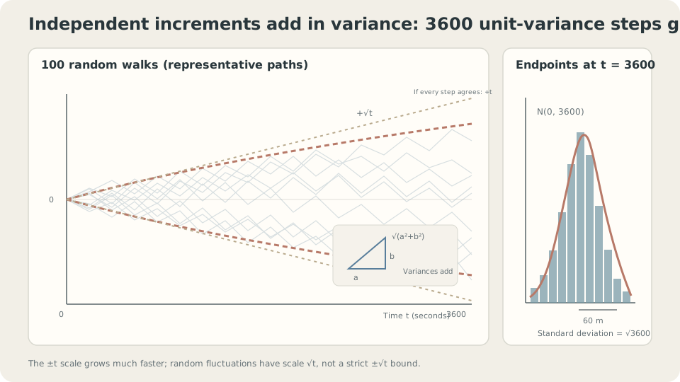
One hundred random-walk trajectories and a square-root-time envelope.

Independent finite-variance steps spread on a square-root scale; the endpoint standard deviation after 3600 steps is 60.

Adding variances and taking the limit

Theorem. Independent centered increments with variance $\sigma^2$ satisfy $\mathbb E[S_n]=0$ and $\operatorname{Var}(S_n)=n\sigma^2$ .

Expand the square:

\mathbb E[S_n^2]=\mathbb E\Big[\sum_i\xi_i^2+\sum_{i\ne j}\xi_i\xi_j\Big]=\sum_i\mathbb E[\xi_i^2]+\sum_{i\ne j}\mathbb E[\xi_i]\,\mathbb E[\xi_j]=n\sigma^2+0 .

Independence factors $\mathbb E[\xi_i\xi_j]$ into the product of means, which is zero. All cross terms disappear. $\square$

Thus RMS distance is $\sigma\sqrt n$ . For iid steps with finite variance, the central limit theorem gives $S_n/\sqrt n\Rightarrow\mathcal N(0,\sigma^2)$ . This is a limiting result for possibly non-Gaussian increments; independence and individual finite variances alone do not establish this iid version.

Brownian limit. Take a step of size $\delta$ every $h$ seconds. At time $t$ , variance is $\delta^2t/h$ . A finite, nonzero limit requires $\delta^2/h$ to stay constant. Set $\delta=\sqrt h$ . The limiting process $W_t$ has these properties:

$W_0=0$ and $W_t\sim\mathcal N(0,t)$ .
Independent stationary increments: $W_t-W_s\sim\mathcal N(0,t-s)$ , independent of the past up to $s$ .
Continuous sample paths.

This is Brownian motion, also called the Wiener process [3]. Over time $h$ , its increment is $\sqrt h\,\varepsilon$ with $\varepsilon\sim\mathcal N(0,1)$ , the basis of the next note’s SDE simulation.

DetailsWhy steps of size h disappear and constant-size steps explode

With t/h steps of size δ, variance is δ²t/h. Setting δ=h gives ht→0; constant δ gives variance tending to infinity; δ=√h gives variance t. The square-root scale warns against interpreting an increment divided by h as ordinary velocity. Almost-sure nowhere differentiability is a separate theorem [3], not proved by this scaling observation. We therefore use increments and stochastic integrals.

Zero mean does not mean returning every time

A zero mean and RMS distance 60 m coexist because left and right displacements cancel across walkers. Rare individuals may travel much farther; one distant outcome does not prove correlation.

For correlated steps, recalculate cross terms. In the specific stationary model that preserves direction with probability $(1+\rho)/2$ , lag- $k$ covariance is $\sigma^2\rho^k$ . For fixed $|\rho|<1$ and large $n$ , variance is approximately $n\sigma^2(1+\rho)/(1-\rho)$ . Merely specifying adjacent correlation does not imply this entire covariance structure. Infinite-variance steps invalidate the RMS calculation.

DetailsVariance for persistent ±1 steps

Start with a symmetric direction and keep it with probability (1+ρ)/2 each step. Then E[ξᵢξᵢ₊ₖ]=ρ^k, so Var(Sₙ)=n+2Σₖ₌₁ⁿ⁻¹(n−k)ρ^k, asymptotically n(1+ρ)/(1−ρ) for fixed |ρ| less than one. Positive persistence increases the coefficient; negative persistence decreases it. At ρ=1, every step keeps its direction and variance is n²; this boundary case must be distinguished from the fixed-ρ large-n limit.

Simulate, then break the assumptions

import numpy as np
rng = np.random.default_rng(0)
def walk(n=3600, rho=0.0, trials=5000):
    keep = rng.random((trials, n)) < (1+rho)/2
    flips = np.where(keep, 1, -1)
    flips[:, 0] = 1
    steps = rng.choice([-1, 1], trials)[:, None] * np.cumprod(flips, axis=1)
    return np.sqrt(np.mean(steps.sum(axis=1)**2))
for rho in [0.0, 0.5, 0.9]:
    print(rho, round(walk(rho=rho)), round(60*np.sqrt((1+rho)/(1-rho))))
# Compare simulated RMS distances with the large-n prediction.

Independence gives RMS near 60. Persistence increases it by approximately $\sqrt{(1+\rho)/(1-\rho)}$ , while multiplying $n$ by four roughly doubles it for fixed $\rho$ . Cauchy steps have no variance: empirical RMS becomes unstable as trials increase, and neither the finite-variance formula nor this Gaussian limit applies.

Check your understanding

References

Grimmett, G., Stirzaker, D. Probability and Random Processes. Oxford University Press, 3rd ed., 2001.
Feller, W. An Introduction to Probability Theory and Its Applications, Vol. 1. Wiley, 3rd ed., 1968.
Mörters, P., Peres, Y. Brownian Motion. Cambridge University Press, 2010.
Einstein, A. Über die von der molekularkinetischen Theorie der Wärme geforderte Bewegung von in ruhenden Flüssigkeiten suspendierten Teilchen. Annalen der Physik 17, 1905.