L2.0 Polling a Small Sample: Minibatch Gradients and Noise

Builds on3 notes

Estimate a population by asking a small sample

A poll surveys a thousand people out of millions and reports a proportion with uncertainty.

For ideal iid Bernoulli sampling, the sample mean is unbiased and its conservative normal-approximation margin is about $1.96\sqrt{0.25/1000}\approx3.1\%$ . Real surveys also involve sampling and response biases. We borrow only the mathematical idea of estimating an average from a random subset.

A full-data training gradient is another average:

g=\nabla L(\theta)=\frac1n\sum_{i=1}^n \nabla \ell\big(f_\theta(x_i),y_i\big).

When the dataset is huge, repeatedly evaluating every example at every update becomes expensive.

Can a small batch provide a useful gradient?
What uncertainty does it introduce?
Does taking more updates automatically remove that uncertainty?

DiscussionQ1

Define the batch estimate. Is its discrepancy bias or variation, and why does moving parameters complicate averaging?

Show the reasoning

At fixed parameters, uniformly sample a batch $S$ of size $B$ and average its per-example gradients:

g_B=\frac1B\sum_{i\in S}\nabla \ell\big(f_\theta(x_i),y_i\big).

Uniform sampling makes the expected average equal the full gradient:

\mathbb E[g_B]=g .

Thus $g_B$ is an unbiased estimate of the empirical gradient under the stated sampling scheme. It is also an approximation, but one with a precise statistical property.

Let $\sigma_g^2=\mathbb E_i\|\nabla\ell_i-g\|^2$ at this parameter value. For independent sampling with replacement,

\mathbb E\lVert g_B-g\rVert^2=\frac{\sigma_g^2}{B}.

Quadrupling $B$ quarters expected squared error, hence halves its root-mean-square magnitude.

Averaging many batches at one fixed parameter reduces uncertainty. SGD instead moves after every batch, so noise changes the position where the next gradient is evaluated. Persistent noise near a minimizer can therefore sustain a nonzero stationary spread.

Noisy downhill directions

Replace the exact local slope in Downhill in Fog: Direction, Step Size, and Gradient Descent with an instrument whose errors average to zero at the queried position.

Each update contains

Gradient drift: the leading local objective decrease is approximately $\eta\|g\|^2$ for a sufficiently small stable step.
Random displacement: its RMS size is approximately $\eta\sigma_g/\sqrt B$ under replacement sampling.

Far from the solution, drift can dominate. If per-example gradients still disagree at the minimizer, noise persists even as their average vanishes. An SDE can approximate some regimes, but its diffusion is generally state-dependent and anisotropic; it is not universally constant isotropic Brownian noise.

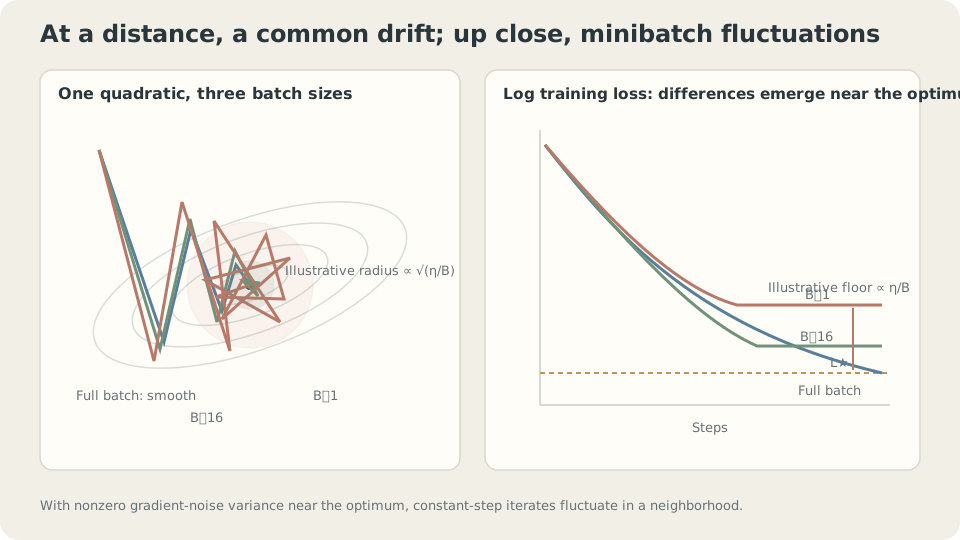
Deterministic descent and random minibatch displacement.

In a suitable local persistent-noise model, stationary parameter spread scales roughly as $\sqrt{\eta/B}$ .

Gradient variance and a stationary floor

For one uniformly selected batch without replacement at fixed parameters, the finite-population correction gives

\mathbb E\lVert g_B-g\rVert^2=\frac{\sigma_g^2}{B}\cdot\frac{n-B}{n-1}.

For $B\ll n$ , the correction is near one. At $B=n$ , it is zero because the entire dataset is the only possible batch.

A solvable floor model: assume quadratic curvature $\lambda>0$ , $0<\eta\lambda<2$ , and conditional centered noise of constant variance $\sigma_g^2/B>0$ at every step. Then

w_{k+1}-w^\star=(1-\eta\lambda)(w_k-w^\star)-\eta\,\xi_k, \qquad \mathbb E[\xi_k]=0,\ \mathbb E[\xi_k^2]=\frac{\sigma_g^2}{B}.

For $e_k=w_k-w^\star$ , the centered cross term vanishes and $\mathbb E[e_{k+1}^2]=(1-\eta\lambda)^2\mathbb E[e_k^2]+\eta^2\sigma_g^2/B$ . At stationarity, solve for the second moment:

\mathbb E\big[(w_\infty-w^\star)^2\big]=\frac{\eta^2\sigma_g^2/B}{1-(1-\eta\lambda)^2}\approx\frac{\eta\,\sigma_g^2}{2\lambda B} \quad\Longrightarrow\quad \mathbb E[L]-L^\star\approx\frac{\eta\,\sigma_g^2}{4B}.

The small- $\eta\lambda$ excess objective is approximately proportional to $\eta/B$ . Curvature cancels at leading order for this scalar objective calculation, but the exact finite-step expression still depends on $\eta\lambda$ ; parameter variance also depends on curvature.

A stable quadratic with persistent centered noise can retain an approximately $\eta/B$ excess-loss floor.

Reducing $\eta$ or increasing $B$ can reduce that floor within this regime. Decreasing-step stochastic approximation uses conditions such as $\sum_k\eta_k=\infty$ and $\sum_k\eta_k^2<\infty$ , together with objective, noise, and stability assumptions; those step-size sums alone do not prove arbitrary training converges.

CautionPossible benefits of noise address another question

This local model studies spread inside one basin. It does not settle every effect of stochastic training.

In nonconvex landscapes, noise may influence transitions between regions. Basin selection and local stationary spread are distinct effects; see One Map, Different Starting Points: Loss Landscapes and Initialization.

Generalization effects of batch size depend on task, optimization, and joint tuning. Even the $\eta/B$ floor is a qualified approximation, not a universal theorem for all training settings.

Sampling assumptions matter

Unbiasedness fixes the current parameters and requires uniform batch selection conditional on them. Fresh independent resampling supports this directly. Random reshuffling followed by sequential batches creates dependence between later batches and current parameters, so per-step conditional unbiasedness is not automatic.

Estimate gradient variability by repeated batches at a fixed checkpoint. This can inform batch comparisons, while remaining local to that checkpoint and sampling scheme.

Estimating a finite empirical gradient does not require dataset rows to be iid; linking that empirical objective to population learning does. Noise may vanish at interpolation solutions, eliminating this particular persistent-noise floor. SGD behavior must be analyzed under the actual assumptions.

Measure variation and the floor

Fixed-parameter experiment: use 120 observations and degree-five features. Repeatedly sample batches without replacement:

import numpy as np
from ml_toy import toy_1d
x,y = toy_1d(n=120,seed=0)
V = np.vander(x,6,increasing=True)
V = V/np.abs(V).max(0)
n = len(x)
w = np.linalg.lstsq(V,y,rcond=None)[0]*.5
g = V.T@(V@w-y)/n
rng = np.random.default_rng(0)
for B in (1,4,16,60,120):
    G = np.array([V[i].T@(V[i]@w-y[i])/B
        for i in (rng.choice(n,B,replace=False) for _ in range(4000))])
    mean_gap = np.linalg.norm(G.mean(0)-g)/np.linalg.norm(g)
    var = ((G-g)**2).sum(1).mean()
    print(B,'relative mean discrepancy',mean_gap,'squared error',var,'B times error',var*B)

B    relative mean gap   squared error   B times error
1    0.0054              0.22878         0.2288
4    0.0303              0.05433         0.2173
16   0.0172              0.01269         0.2030
60   0.0015              0.00201         0.1207
120  0.0000              0.00000         0.0000

Finite Monte Carlo discrepancies fluctuate around the theoretical zero mean difference. The full-data batch agrees exactly. The experiment illustrates unbiasedness; a small discrepancy in one run does not by itself prove it.

Small batches approximately follow $1/B$ . At half and full dataset sizes, finite-population correction matters. Compare the measured $B$ -scaled values with $\sigma_g^2(n-B)/(n-1)$ rather than a constant alone.

Stationary behavior: orthogonalize features so full-batch conditioning is simple. Start at the empirical optimum and average the tail of a long run:

Q = np.linalg.qr(np.vander(x,4,increasing=True))[0]*np.sqrt(n)
L = lambda w:((Q@w-y)**2).mean()
w_opt = np.linalg.lstsq(Q,y,rcond=None)[0]
for eta in (.02,.05,.1):
    for B in (1,4,16):
        rng = np.random.default_rng(1)
        w = w_opt.copy()
        tail = []
        for t in range(60000):
            idx = rng.choice(n,B,replace=False)
            w -= eta*(Q[idx].T@(Q[idx]@w-y[idx]))/B
            if t>=50000: tail.append(L(w))
        delta = np.mean(tail)-L(w_opt)
        print(eta,B,'excess MSE',delta,'scaled',delta/(eta/B))

eta   B   excess MSE   excess/(eta/B)
.02   1   .00138       .0692
.02   4   .00033       .0660
.02   16  .00007       .0524
.05   1   .00385       .0771
.05   4   .00084       .0673
.05   16  .00018       .0560
.10   1   .00913       .0913
.10   16  .00037       .0596

The scaled excess stays within a moderate range, consistent with approximate $\eta/B$ behavior. State-dependent noise, finite-population correction, finite-step effects, and finite tail averaging prevent an exact common coefficient.

Similar ratios can suggest comparable local noise levels, but changing rate and batch together also changes update count, stability, and computation. Linear rate scaling with batch size is an empirical strategy to test within a regime, not an unrestricted equivalence.

With ill-conditioned raw features and a limited run, a larger stable rate can yield lower loss simply by making more progress before stationarity. That transient comparison does not contradict the local floor calculation.

A stationary-floor calculation does not describe every point on a still-improving training curve.

Inspect trajectories and rate-reduction comparisons. A plateau is evidence to investigate, not proof of a noise floor: capacity, saturation, numerical issues, and other optimization effects can also produce one.

Vary rate and batch size

Compare the approximate ratio effect while checking stability and transient progress.

Check your understanding

References

Robbins, H., Monro, S. A Stochastic Approximation Method. Annals of Mathematical Statistics 1951.
Bottou, L., Curtis, F., Nocedal, J. Optimization Methods for Large-Scale Machine Learning. SIAM Review 2018.
Smith, S., Kindermans, P.-J., Ying, C., Le, Q. Don’t Decay the Learning Rate, Increase the Batch Size. ICLR 2018.