M2.4 One More Look Halfway Through: Higher-Order Methods

Builds on2 notes

The same bend, one extra reading

In M2.3, infrequent navigation updates gave an endpoint error near 486 m on a quarter-circle of radius 2 km. Updating every 10 rather than 30 seconds reduced it to about 161 m, at three times the evaluation cost.

Euler treats velocity as constant over each step, like a rectangle under a curve. An endpoint estimate suggests a trapezoid; a midpoint estimate suggests a velocity closer to the step average. Can this extra reading recover the acceleration term Euler missed?

DiscussionQ1

How do we write a midpoint reading as an update, and what comparison fairly accounts for its cost?

Show the reasoning

First predict a midpoint with a half Euler step, evaluate velocity there, then take a full step from the original position using that velocity:

k_1=v(x_n,t_n),\qquad k_2=v\!\big(x_n+\tfrac{h}{2}k_1,\;t_n+\tfrac h2\big),\qquad x_{n+1}=x_n+h\,k_2 .

This is explicit midpoint. Heun’s method instead predicts an endpoint with Euler and averages the velocities at the original and predicted positions:

k_1=v(x_n,t_n),\qquad k_2=v(x_n+h\,k_1,\;t_n+h),\qquad x_{n+1}=x_n+\tfrac h2(k_1+k_2).

Euler uses the initial velocity, midpoint uses the predicted midpoint velocity, and Heun averages the two endpoint evaluations.

Compare equal numbers of function evaluations (NFE). Euler costs one per step; Heun and midpoint cost two. For example, over a three-minute interval, twelve Euler steps of 15 seconds and six midpoint steps of 30 seconds both cost twelve evaluations.

Tangent versus chord

On a circular arc, Euler follows the initial tangent and misses the exact endpoint by $O(h^2)$ locally.

The exact midpoint tangent is parallel to the chord and better approximates net displacement. But numerical midpoint uses a predicted midpoint, and its endpoint need not lie exactly on the circle. Taylor expansion must verify the improvement suggested by this picture.

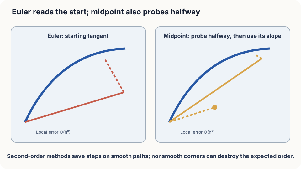
Initial tangent in Euler compared with the midpoint slope on a curved path.

An extra field evaluation provides second-order accuracy on smooth problems.

Match the quadratic term

Assume sufficient smoothness and bounded relevant derivatives. Starting from the exact position, the acceleration defined previously gives

x_{t+h}=x_t+h v_t(x_t)+\tfrac{h^2}{2}a_t(x_t)+O(h^3).

Heun first. The predicted endpoint is $\tilde x_{t+h}=x_t+hv_t(x_t)$ . Expand in both position and time:

\begin{aligned} v_{t+h}(\tilde x_{t+h}) &=v_t(x_t)+h\partial_t v_t(x_t) +h\nabla_xv_t(x_t)\,v_t(x_t)+O(h^2)\\ &=v_t(x_t)+h a_t(x_t)+O(h^2). \end{aligned}

The average velocity is consequently $v_t(x_t)+\frac h2a_t(x_t)+O(h^2)$ . Multiplying by $h$ gives

x_t+\tfrac h2\big(v_t(x_t)+v_{t+h}(\tilde x_{t+h})\big) =x_t+h v_t(x_t)+\tfrac{h^2}{2}a_t(x_t)+O(h^3).

This matches the exact solution through the quadratic term. At the predicted half-step, midpoint likewise evaluates $v_t(x_t)+\frac h2a_t(x_t)+O(h^2)$ and matches the same terms.

Global error. The propagation argument from M2.3 now accumulates $O(h^3)$ local defects over $T/h$ steps, giving $O(h^2)$ globally. Halving $h$ therefore reduces the leading error by approximately four, compared with two for Euler.

Under appropriate consistency and stability assumptions, local error $O(h^{p+1})$ leads to global error $O(h^p)$ : order $p$ . Euler has order one; Heun and midpoint have order two. Classical RK4 has order four and uses four evaluations per step [1,2].

DetailsThe numerical integration view when velocity depends only on time

If v=v(t), the solution integrates v over the step. Euler uses the left rectangle h·v(t), with leading exact-minus-numerical error (h²/2)v′. Midpoint uses h·v(t+h/2); expansion about the midpoint m cancels odd powers, leaving leading exact-minus-numerical error (h³/24)v″(m). Heun uses the trapezoid (h/2)[v(t)+v(t+h)], whose numerical-minus-exact error is (h³/12)v″(m). These are leading terms in the time-only case. Position dependence introduces additional terms, so these constants do not generally predict the ratio of ODE solver errors.

When does the extra reading help?

For the smooth bend, midpoint at roughly 30-second steps gives about 7 m error and Heun about 23 m, far below the more expensive 10-second Euler estimate. The extra evaluation cancels a leading error term, changing its order rather than merely halving its coefficient.

The benefit depends on several conditions:

Smoothness: bounded derivatives justify the remainder estimates. Discontinuities or corners require separate analysis, sometimes including event location.
Budget: with $E$ evaluations, second-order error behaves like $C_2(2T/E)^2$ , while Euler behaves like $C_1T/E$ . The asymptotic $E^{-2}$ improvement need not dominate at extremely coarse steps or tiny budgets.
Stability: higher order does not permit arbitrary step sizes. For $\dot x=-kx$ , both methods have amplification $1-hk+(hk)^2/2$ , whose decay interval on the negative real axis is still $0<hk<2$ .

Compare equal evaluation budgets

import numpy as np
R, v = 2000.0, 60/3.6
T = (np.pi/2)*R/v
def u(x):
    r = np.hypot(*x)
    return v*np.array([-x[1], x[0]])/r
def run(method, nfe):
    steps = nfe if method == 'euler' else nfe//2
    h = T/steps
    x = np.array([R, 0.0])
    for _ in range(steps):
        k1 = u(x)
        if method == 'euler':
            x = x + h*k1
        else:
            x = x + h*u(x + 0.5*h*k1)
    return np.linalg.norm(x - np.array([0.0, R]))
for nfe in [12, 38, 126]:
    print(nfe, round(run('euler', nfe)), round(run('midpoint', nfe), 1))
# Compare errors using exactly the same evaluation budget.

On this smooth example, midpoint is substantially more accurate at equal NFE, with an increasing advantage as the budget grows. A path with an unresolved right-angle corner violates the smoothness assumptions: the crossing step can incur an $O(h)$ defect and sharply reduce the advantage. The exact result depends on how the corner and crossing event are modeled.

Check your understanding

References

Hairer, E., Nørsett, S. P., Wanner, G. Solving Ordinary Differential Equations I: Nonstiff Problems. Springer, 2nd ed., 1993.
Butcher, J. C. Numerical Methods for Ordinary Differential Equations. Wiley, 3rd ed., 2016.