U3.1 How Do We Measure the Velocity Changes Euler Misses?

Builds on4 notes

Euler checks velocity at the start of a step and freezes both direction and speed. Turning causes deviation, but even straight motion can overshoot or undershoot if speed changes.

We therefore need more than geometric curvature: how much velocity change did Euler miss, and what endpoint error can it cause?

Can we quantify velocity variation along a trajectory and bound its numerical error?

Interactive demo. Keep the field and starting point fixed while changing Euler’s step count. The fine numerical reference remains unchanged; coarse steps cut across turns and alter the endpoint.

What does one Euler step omit?

Follow the standard local-to-global Euler analysis [1].

Consider an exact ODE trajectory:

\frac{\mathrm d x_t}{\mathrm d t}=v_t(x_t).

Its exact displacement is

x_{t+h}=x_t+\int_t^{t+h}v_\tau(x_\tau)\,\mathrm d\tau.

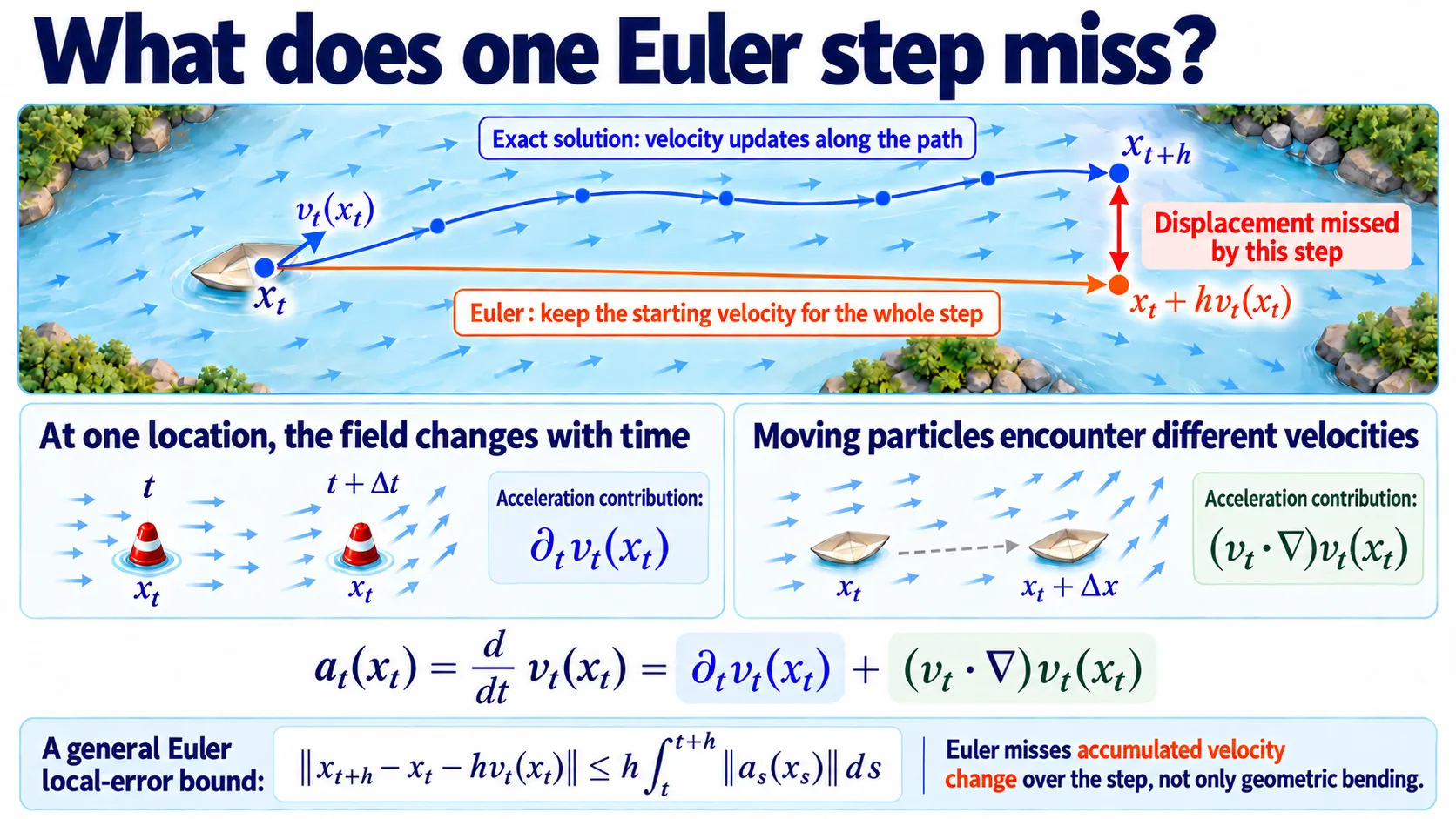
Euler replaces the entire interval’s velocity with its initial value, yielding $x_t+hv_t(x_t)$ .

Define acceleration along the exact trajectory:

a_s(x_s):=\frac{\mathrm d}{\mathrm ds}v_s(x_s).

Integrating acceleration gives the intermediate velocity change:

v_\tau(x_\tau) =v_t(x_t)+\int_t^\tau \frac{\mathrm d}{\mathrm ds}v_s(x_s)\,\mathrm ds =v_t(x_t)+\int_t^\tau a_s(x_s)\,\mathrm ds.

Substitute this into the displacement and exchange the order of integration:

\begin{aligned} x_{t+h} &=x_t+h\,v_t(x_t) +\int_t^{t+h}\int_t^\tau a_s(x_s)\,\mathrm ds\,\mathrm d\tau\\ &=x_t+h\,v_t(x_t) +\int_t^{t+h}(t+h-s)\,a_s(x_s)\,\mathrm ds. \end{aligned}

The final integral is the omitted local remainder. Its norm satisfies

\left\|x_{t+h}-x_t-hv_t(x_t)\right\| \le h\int_t^{t+h}\|a_\tau(x_\tau)\|\,\mathrm d\tau.

Expand acceleration using the chain rule:

\begin{aligned} a_t(x_t)&=\frac{d}{dt}v_t(x_t)\\ &=\underbrace{\partial_t v_t(x_t)}_{\text{field changes with time}} +\underbrace{(v_t\cdot\nabla)v_t(x_t)}_{\text{particle changes location}}. \end{aligned}

One contribution comes from the field changing at a fixed position. The other comes from a particle moving through a spatially varying field. Their sum is the experienced acceleration.

SupplementAcceleration is not geometric curvature

Let $\rho_t$ be speed, $T_t$ the unit tangent, and $s$ arc length. Geometric curvature is

\kappa_t=\left\|\frac{\mathrm dT_t}{\mathrm ds}\right\|,

It measures direction change per unit arc length. Acceleration instead decomposes as

a_t(x_t) =\frac{\mathrm d\rho_t}{\mathrm dt}T_t +\rho_t^2\kappa_tN_t.

The tangential term changes speed; the normal term changes direction. A straight path can have zero curvature but nonzero acceleration. Euler’s bound uses the full acceleration.

Constant-speed straight motion has zero acceleration and makes every Euler step exact. This is the trajectory property we seek, rather than straightness without a speed condition.

Euler's missed velocity variation and the temporal and spatial sources of acceleration.

Figure: Euler retains the initial arrow while exact motion updates it continuously, through both temporal and spatial changes.

How does one-step error reach the endpoint?

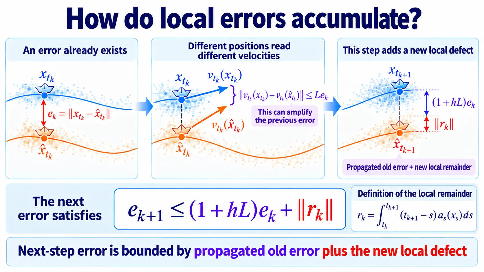
A displaced numerical state also queries velocity at the wrong location. On a uniform grid, define its distance from the exact state:

e_k:=\|x_{t_k}-\hat x_{t_k}\|.

The exact update is

x_{t_{k+1}} =x_{t_k}+h\,v_{t_k}(x_{t_k})+r_k,

with local remainder

r_k=\int_{t_k}^{t_{k+1}}(t_{k+1}-s)a_s(x_s)\,\mathrm ds,\qquad \|r_k\|\le h\int_{t_k}^{t_{k+1}}\|a_s(x_s)\|\,\mathrm ds.

while Euler uses

\hat x_{t_{k+1}} =\hat x_{t_k}+h\,v_{t_k}(\hat x_{t_k}).

Subtract:

x_{t_{k+1}}-\hat x_{t_{k+1}} =(x_{t_k}-\hat x_{t_k}) +h\big(v_{t_k}(x_{t_k})-v_{t_k}(\hat x_{t_k})\big) +r_k.

The terms represent previous displacement, velocity mismatch from that displacement, and new local remainder. Control the second using a spatial Lipschitz assumption.

SupplementLipschitz continuity controls nearby velocity differences

Assume that at every time and for all positions,

\|v_t(x)-v_t(y)\|\le L\|x-y\|,

Then the field is $L$ -Lipschitz in space. Two particles distance $\delta$ apart see velocities differing by at most $L\delta$ . Larger $L$ allows stronger sensitivity to position errors.

This compares positions at the same time. Temporal variation is already included in the local remainder.

Take norms and apply the triangle inequality:

\begin{aligned} e_{k+1} &\leq\|x_{t_k}-\hat x_{t_k}\|\\ &\quad+h\|v_{t_k}(x_{t_k})-v_{t_k}(\hat x_{t_k})\|\\ &\quad+\|r_k\|. \end{aligned}

The first term is $e_k$ , and Lipschitz continuity bounds the second by $hLe_k$ . Therefore

\begin{aligned} e_{k+1} &\le e_k+hLe_k+\|r_k\|\\ &=(1+hL)e_k+\|r_k\|. \end{aligned}

Previous error may grow by $(1+hL)$ , and each step adds its own remainder.

Local Euler remainders accumulate while spatial sensitivity can amplify earlier displacement.

Figure: an earlier displacement changes the next velocity query, propagating old error while new local error is added.

Unroll from $e_0=0$ through $N=1/h$ steps:

\begin{aligned} e_N &\le \sum_{k=0}^{N-1}(1+hL)^{N-1-k}\|r_k\|\\ &\le e^L h\sum_{k=0}^{N-1} \int_{t_k}^{t_{k+1}}\|a_s(x_s)\|\,\mathrm ds\\ &=e^L h\int_0^1\|a_t(x_t)\|\,\mathrm dt. \end{aligned}

Use $(1+hL)^N\leq e^L$ , a discrete Grönwall estimate over the unit interval.

For each shared initial point,

\boxed{ \|x_1-\hat x_1\| \le e^L h\int_0^1\|a_t(x_t)\|\,\mathrm dt }

The bound separates three factors:

Step size $h$ : refinement reduces this upper bound linearly.
Integrated acceleration: accumulated velocity variation includes turns, acceleration, and deceleration.
Amplification $e^L$ : field sensitivity can magnify local displacement.

Euler error is controlled by integrated trajectory acceleration, rather than geometric curvature alone.

DetailsFrom trajectory error to Wasserstein error: model and solver contributions

Practical generation uses a learned field and then discretizes it. Endpoint error has two distinct sources:

Modeling error: the learned field differs from the ideal one.
Discretization error: Euler approximates the fixed learned ODE.

Start three constructions from the same random source:

\frac{\mathrm dX_t}{\mathrm dt}=v_t(X_t),\qquad \frac{\mathrm d\widetilde X_t}{\mathrm dt}=v_\theta(\widetilde X_t,t),\qquad \widehat X_{t_{k+1}} =\widehat X_{t_k}+h\,v_\theta(\widehat X_{t_k},t_k).

Let $X_1$ be the ideal endpoint, $\widetilde X_1$ the exactly integrated learned endpoint, and $\widehat X_1$ its Euler approximation. Their laws are

X_1\sim p_1,\qquad \widetilde X_1\sim\widetilde p_1,\qquad \widehat X_1\sim\widehat p_1.

Wasserstein distance minimizes squared transport cost over couplings:

W_2^2(q,r) =\inf_{\Gamma\in\Pi(q,r)} \mathbb E_{(Y,\widehat Y)\sim\Gamma} \|Y-\widehat Y\|^2.

Shared starting points provide legal endpoint couplings. The triangle inequality gives

\begin{aligned} W_2(p_1,\widehat p_1) &\leq\underbrace{W_2(p_1,\widetilde p_1)}_{\text{modeling error}}\\ &\quad+\underbrace{W_2(\widetilde p_1,\widehat p_1)}_{\text{discretization error}}. \end{aligned}

First term: learned versus ideal velocity

Define the population velocity error:

\mathcal E_v :=\int_0^1 \mathbb E_{X_t\sim p_t} \big[\|v_\theta(X_t,t)-v_t(X_t)\|^2\big]\,\mathrm dt.

Assume the learned field is $L$ -Lipschitz. Add and subtract its value at the ideal position:

\begin{aligned} \frac{\mathrm d}{\mathrm dt}\|\widetilde X_t-X_t\| &\le \|v_\theta(\widetilde X_t,t)-v_t(X_t)\|\\ &\le \underbrace{\|v_\theta(\widetilde X_t,t)-v_\theta(X_t,t)\|}_{\le L\|\widetilde X_t-X_t\|} +\underbrace{\|v_\theta(X_t,t)-v_t(X_t)\|}_{\text{velocity prediction error}}. \end{aligned}

Write the instantaneous prediction error as

\delta_t:=\|v_\theta(X_t,t)-v_t(X_t)\|.

Grönwall accumulates it to the endpoint:

\|\widetilde X_1-X_1\| \le e^L\int_0^1\delta_t\,\mathrm dt.

Square, average, and use Cauchy–Schwarz:

\begin{aligned} \mathbb E\|\widetilde X_1-X_1\|^2 &\le e^{2L}\, \mathbb E\left[\left(\int_0^1\delta_t\,\mathrm dt\right)^2\right]\\ &\le e^{2L}\int_0^1\mathbb E[\delta_t^2]\,\mathrm dt =e^{2L}\mathcal E_v. \end{aligned}

Since the paired endpoints define a coupling,

W_2(p_1,\widetilde p_1) \le e^L\sqrt{\mathcal E_v}.

This term remains even with exact numerical integration.

Second term: Euler versus the learned ODE

Now hold the learned field fixed and define its trajectory acceleration:

\widetilde a_t(\widetilde X_t) :=\frac{\mathrm d}{\mathrm dt}v_\theta(\widetilde X_t,t),\qquad \widetilde A(X_0) :=\int_0^1\|\widetilde a_t(\widetilde X_t)\|\,\mathrm dt.

Apply the pathwise Euler estimate to the shared-source coupling:

\begin{aligned} W_2^2(\widetilde p_1,\widehat p_1) &\le\mathbb E\|\widetilde X_1-\widehat X_1\|^2\\ &\le e^{2L}h^2\mathbb E[\widetilde A(X_0)^2], \end{aligned}

Thus

W_2(\widetilde p_1,\widehat p_1) \le e^L h \Big(\mathbb E[\widetilde A(X_0)^2]\Big)^{1/2}.

This is the finite-step contribution, which decreases with refinement under the stated regularity.

Combining the terms gives

\boxed{ W_2(p_1,\widehat p_1) \le e^L \left[ \sqrt{\mathcal E_v} +h\Big(\mathbb E[\widetilde A(X_0)^2]\Big)^{1/2} \right]. }

Increasing steps reduces numerical error but cannot remove a fixed model error. Conversely, small regression error does not ensure accurate coarse sampling if the learned trajectory has substantial velocity variation.

These shared-source couplings only give upper bounds. Small Wasserstein distance does not imply small error for a particular pairing of individual trajectories; the distance may find a cheaper pairing.

Check your understanding

References

Hairer, E., Nørsett, S. P., Wanner, G. Solving Ordinary Differential Equations I: Nonstiff Problems. Springer.
Liu, X., Gong, C., Liu, Q. Flow Straight and Fast: Learning to Generate and Transfer Data with Rectified Flow. ICLR 2023.