U7.5 實作：同一個 base distribution，能被 guidance 帶到哪裡？

本篇重用4 篇

• U7.1不重新訓練，怎麼取得這次要求的引導方向？
• U7.2既要像資料，又要 reward 高：我們真正想抽哪個 distribution？
• U7.3Reward 只會打分、不會給方向，還能怎麼引導？
• M3.3山谷裡隨機走的人群：Langevin Dynamics 與 Stationary Distribution

先建立一個每一項都算得出來的 base distribution

這次不先訓練 neural network。我們用四個 Gaussian modes 建立 2D base distribution，讓 score、condition 與 reward-tilted ground truth 都能直接計算。若方法連這個 toy 的 target 都對不上，換到大型 diffusion model 後更難知道誤差來自 guidance、network，還是 sampler。

令

$$p_{\mathrm{data}}(x) =\frac14\sum_{j=1}^4 \mathcal N(x;\mu_j,\sigma^2I), \qquad \mu_j\in\{(-2,-2),(-2,2),(2,-2),(2,2)\},$$

並取 $\sigma=0.45$。把上方兩個 modes 定成 condition $c=1$，下方兩個 modes 定成 $c=0$。

對每個 $x$，先算未 normalization 的 component densities $\rho_j(x)$ 與 responsibilities：

$$r_j(x)=\frac{\rho_j(x)}{\sum_{\ell=1}^4\rho_\ell(x)}.$$

Gaussian mixture 的 score 是每個 component score 按 posterior responsibility 加權：

$$s(x)=\sum_{j=1}^4r_j(x)\frac{\mu_j-x}{\sigma^2}.$$

這就是 U1.3 的 posterior average，在一個不需要網路的例子裡直接算出來。程式可先寫成：

import math
import torch

SIGMA = 0.45
MUS = torch.tensor([[-2., -2.], [-2., 2.], [2., -2.], [2., 2.]])
TOP = torch.tensor([False, True, False, True])

def log_components(x, mask=None):
    mus = MUS if mask is None else MUS[mask]
    d2 = ((x[:, None, :] - mus[None, :, :]) ** 2).sum(-1)
    return -0.5 * d2 / SIGMA**2

def mixture_score(x, mask=None):
    mus = MUS if mask is None else MUS[mask]
    log_rho = log_components(x, mask)
    resp = torch.softmax(log_rho, dim=1)
    return (resp[..., None] * (mus[None] - x[:, None]) / SIGMA**2).sum(1)

mixture_score(x) 是 unconditional score；mixture_score(x, TOP) 是 $c=1$ 的 conditional score。兩者都在同一組 $x$ 上評估，才有辦法比較方向。

步驟 1：親手驗證 classifier gradient 就是兩個 score 的差

Condition probability 可以直接由 mixture components 算：

$$p(c=1\mid x) =\frac{\sum_{j:\,\mu_{j,2}=2}\rho_j(x)}{\sum_{j=1}^4\rho_j(x)}.$$

用 autograd 對 $\log p(c=1\mid x)$ 求 gradient，再和

$$s(x\mid c=1)-s(x)$$

逐點比較。在 $[-4,4]^2$ 的 regular grid 上畫兩個 vector fields，並回報 maximum absolute error。浮點誤差之外，兩者應該一致；這一步是在數值上檢查 U7.1 的 Bayes identity，不是在比較兩個近似 network。

步驟 2：$w=0,1,3$ 真的在抽不同的 distributions

用 exact scores 做 Langevin sampling：

$$x^{(m+1)}=x^{(m)}+\frac h2\widetilde s_w(x^{(m)})+\sqrt h\,\xi^{(m)}, \qquad \xi^{(m)}\sim\mathcal N(0,I),$$

其中

$$\widetilde s_w(x) =s(x)+w\big[s(x\mid c=1)-s(x)\big].$$

從同一批 initial particles 出發，固定 $h$、burn-in 與總步數，只換 $w\in\{0,1,3\}$。畫三張 scatter plots，並報告：

• 上方 modes 的總 mass；
• 左上／右上兩個 modes 各自的 mass；
• samples 的 covariance trace，作為 spread 的簡單量測。

$w=0$ 應回到四個 modes 的 base distribution；$w=1$ 應只保留上方兩個 modes，且左右比例仍接近 $1:1$；$w=3$ 會更強地排斥下方區域，但 finite-step Langevin 與有限 samples 下不一定讓任何單一 metric 都單調改善。這一步的重點是：guidance strength 改的是 target score，不只是 convergence speed。

步驟 3：建立一個不提供 gradient 的 reward

接著拿掉 condition，改成只能回傳分數的 reward。令

$$R(x)=\mathbf 1\{\|x-(3.0,3.0)\|\le0.55\}.$$

這個事件落在右上 mode 的外側尾端：base model 偶爾能抽到，但不常見；reward 只有 0 或 1，在邊界上也沒有實作用途的 gradient。

取 $\lambda\in\{1,3,6\}$，在 dense grid 上直接 normalization：

$$p_R(x)\propto p_{\mathrm{data}}(x)e^{\lambda R(x)}.$$

這張 grid density 是後面比較的 ground truth。記錄 target event probability、四個 modes 的 mass 與 $\mathbb E_{p_R}[\log p_{\mathrm{data}}(x)]$；後者用來看 reward 提高時，data fidelity 掉了多少。

步驟 4：Best-of-$N$ 與 tempering SMC

Best-of-$N$。 每組從 base mixture 獨立抽 $N$ 個 samples，輸出 reward 最大者；若並列，用 uniform tie-breaking。掃 $N\in\{4,16,64,256\}$，重複多個 seeds。除了 best reward，也要畫被選 samples 的 mode distribution——binary reward 常會產生大量 ties，tie-breaking 仍會影響 diversity。

Tempering SMC。 維持 $M$ 個 particles，令 $0=\lambda_0<\lambda_1<\cdots<\lambda_K=\lambda$。從 $\lambda_{k-1}$ 走到 $\lambda_k$ 時，incremental weight 是

$$\omega_k^{(i)} \propto \exp\Big((\lambda_k-\lambda_{k-1})R(x^{(i)})\Big).$$

Normalize weights 後算 effective sample size

$$\operatorname{ESS}=\frac{1}{\sum_i(\bar\omega_k^{(i)})^2}.$$

若 ESS 小於 $M/2$，做 multinomial 或 systematic resampling。Resampling 後，用 random-walk Metropolis 做幾步 rejuvenation；proposal 只需要算

$$\log p_{\mathrm{data}}(x)+\lambda_kR(x),$$

不需要 reward gradient。這個 toy 的 base log-density 可精確計算，因此 acceptance ratio 也能精確寫出來。

課堂提問Q1

Best-of-$N$ 用 $N$ 次 reward evaluations，SMC 卻在每個 temperature、每次 Metropolis proposal 都要重新評分。只固定 particle 數量 $M=N$，就能說哪個方法比較有效率嗎？

先想一想，再展開看整理後的答案

不行。相同 particle 數量不代表相同 test-time compute。SMC 重複使用 particles，代價是多次 reward evaluations、base-density evaluations 與 proposal steps；在真正 diffusion／flow model 裡，還可能多出 generator calls。

至少要同時報告：

• reward evaluations；
• diffusion／flow model evaluations；
• wall-clock time；
• 最終 reward、base log-density 與 diversity。

公平的第一個比較，是固定 reward-evaluation budget $B$。Best-of-$N$ 用 $N=B$；SMC 則選 $M$、temperatures 與 rejuvenation steps，使總 evaluations 接近 $B$。第二個比較再固定 model evaluations，因為有些 reward 很便宜、生成很貴，有些 scientific simulator 則剛好相反。

Test-time scaling 沒有脫離計算預算。 方法的價值在於同一份額外 compute 是否被更有效地轉成 target mass，而不是 particles 看起來比較多。

步驟 5：不要只報最高 reward

每個設定至少報五個量：

1. mean reward 與 event hit rate；
2. mean base log-density；
3. 四個 modes 的 coverage；
4. sample covariance 或 pairwise distance；
5. reward evaluations 與 model／density evaluations。

再把 empirical histogram 和步驟 3 的 exact $p_R$ 比較。Best-of-$N$ 的輸出 distribution 通常不等於 $p_R$；tempering SMC 在 particles、temperatures 與 MCMC mixing 都增加時，才應該逐漸靠近 grid ground truth。若 reward 高但 base log-density 暴跌，或 samples 全部變成同一個點，就不能只用「alignment 變好」收掉結果。

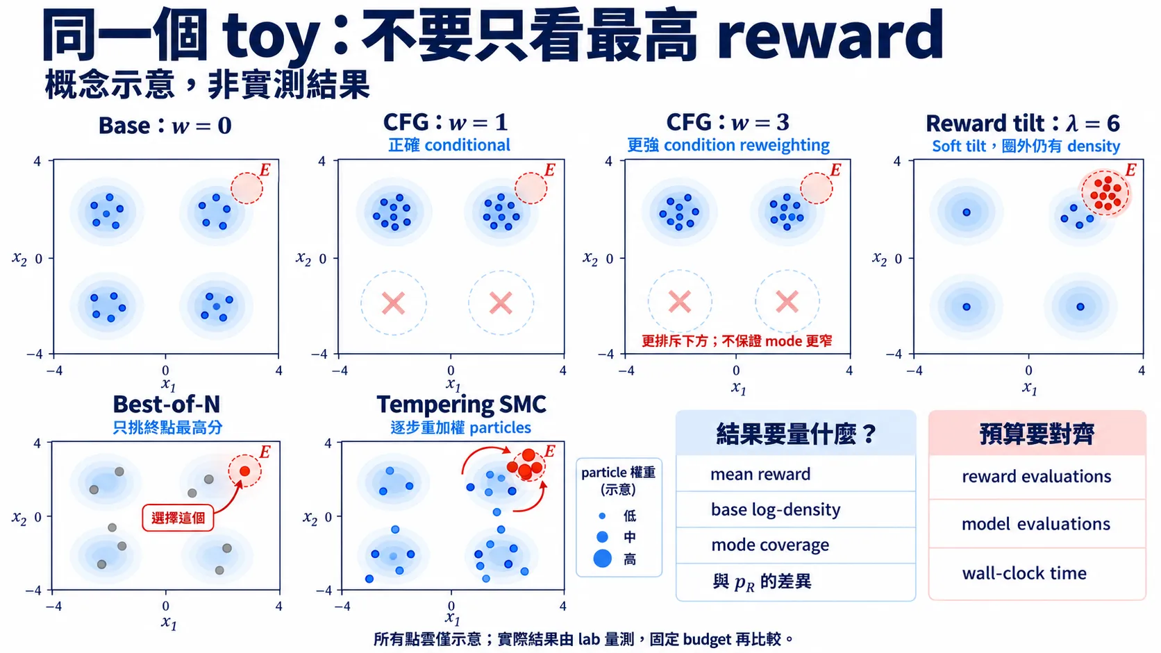
圖：target 與 sampling 機制的概念示意，並非實驗結果。較大的 CFG 權重不保證每個 mode 都變窄；實際的 reward、base fidelity、coverage 與 budget 需由 lab 量測。

作業

1. 把 binary reward 換成 smooth reward。 使用 $R(x)=-\|x-(3,3)\|^2$，比較 exact tilted score $s(x)+\lambda\nabla R(x)$、Best-of-$N$ 與 SMC。固定 reward-evaluation budget 後，哪一種方法在 $\lambda$ 增大時最先失去 mode coverage？
2. 把 reward 移到兩個 modes 之間。 將 reward center 設為 $(0,2)$。高 reward 區域的 base density 很低；畫出 $\lambda$ 增加時 mean reward 與 mean base log-density 的 trade-off。這是 reward hacking 的最小版本。
3. 故意讓 resampling 太早。 把 ESS threshold 從 $M/2$ 改成 $0.9M$，並拿掉 rejuvenation。畫 particle ancestors 的數量隨 temperature 變化，確認 particle degeneracy 如何讓 diversity 提前消失。
4. （選）改成 source-space search。 用一個固定的 invertible 2D map $G$ 將 $z\sim\mathcal N(0,I)$ 送到四 modes，在 $z$ 空間做 random-walk Metropolis 與 parallel tempering，對照 data-space proposals 的 acceptance rate 與跨 mode 次數。

消化一下

想一想

步驟 1 中，若 mixture_score(x, TOP) - mixture_score(x) 與 autograd 的 classifier gradient 對不上，最先該檢查什麼？ Langevin step size。 Conditional mixture 是否只在上方 components 內重新 normalization，以及兩邊是否在同一批 $x$ 上計算。 Reward strength $\lambda$。

看解答

想一想

為什麼 $w=3$ 的 samples 不能拿來當 $p(x\mid c=1)$ 的 ground truth？ 因為 $w=3$ 需要三個 classifiers。 因為本篇 convention 下 $w=1$ 才是 conditional score；$w=3$ 已經對 condition 做額外 power reweighting。 因為 Langevin 只能使用整數 $w$。

看解答

想一想

Tempering SMC 中 ESS 很低表示什麼？ Particles 已經均勻覆蓋 target。 少數 particles 佔了大部分 normalized weight，population 即將失去有效的多樣性。 Reward 沒有被呼叫。

看解答

參考文獻

1. Ho, J., Salimans, T. Classifier-Free Diffusion Guidance. 2022.（步驟 1–2 的 CFG identity。）
2. Singhal, R. et al. A General Framework for Inference-time Scaling and Steering of Diffusion Models. ICML 2025.（Particle-based FK steering。）
3. Kim, S., Kim, M., Park, D. Test-time Alignment of Diffusion Models without Reward Over-optimization. 2025.（Tempering SMC。）