U1.1 Choosing a Path: The Forward Process

Builds on2 notes

We know how to move in one direction

The previous note suggested choosing a path before designing regression targets. How should we choose it?

A path from pure noise to an image is still difficult: we do not know what the noise should become in the next step.

What about the opposite direction? Start with a real image and add a small Gaussian perturbation. Repeat until little image structure remains. Data to noise is a direction we know how to construct.

Think of shuffling an ordered deck. Repeated small shuffles make it random; restoring an arbitrary random deck in one move is hard. Undoing a small amount of disorder sounds more manageable.

Diffusion uses this familiar direction to construct many small corruption steps and learn how to reverse them. A difficult generation task becomes a sequence of denoising problems.

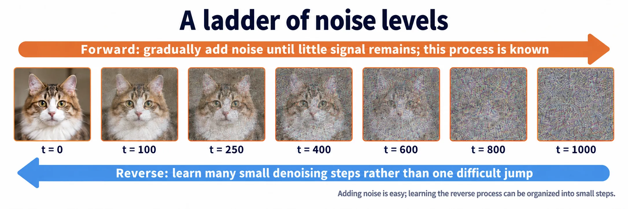
Seven frames of a cat image, gradually corrupted from clean data at t=0 to nearly pure noise at t=1000.

Figure: a ladder of noise levels. Moving right only requires Gaussian draws, scaling, and addition. We want to learn the steps going left.

Let us describe this construction mathematically.

$x_0$ is a real image sampled from $p_{\text{data}}$ . The state after $t$ corruption steps is $x_t$ , where $t$ is also called time. The endpoint $x_T$ should be nearly pure noise.

The path from $x_0$ to $x_T$ is the forward process. We design it ourselves, so we can choose a convenient construction.

We want to answer these questions:

Does the endpoint really approach pure noise?
What is the distribution of $x_t$ given $x_0$ ?
What do we need to reverse a step, and how do we do it?

This note answers the first two. The required reverse-step information appears in U1.2 and U1.3; sampling is developed in U1.4.

What should the forward process accomplish?

Repeated small noise additions give us a direction. To turn it into a usable method, we should work backward from what we need.

First, the endpoint must have a distribution we can sample, here $\mathcal N(0,I)$ . Reverse generation needs a starting state. An inaccessible terminal distribution would prevent us from even beginning.

Second, we want to calculate the distribution at any time $t$ , preferably without simulating all preceding steps. A Gaussian closed form for $q(x_t\mid x_0)$ would be particularly convenient.

Here $q$ denotes the probability law induced by our forward construction. The conditional density $q(x_t\mid x_0)$ describes where the process lies after $t$ steps when the clean starting image $x_0$ is known.

The endpoint is simply the special case $t=T$ , so a general formula would answer both requirements.

Imagine traveling from Taipei to Pingtung by either the west or east coast. The start is $x_0$ and intermediate stops are $x_t$ . A one-step transition describes the next stop; $q(x_t\mid x_0)$ describes the location after $t$ legs, regardless of the intermediate route.

Ignoring the route means integrating over every possible intermediate state:

q(x_t\mid x_0)=\int q(x_1,\dots,x_t\mid x_0)\;\mathrm dx_1\cdots\mathrm dx_{t-1}.

The joint density describes a particular sequence of intermediate states given $x_0$ . Integration sums their contributions while keeping only the final state.

Can we deliberately design the process so this integration is easy?

First design: let the next step depend only on the present

Require each transition to depend only on the preceding state:

q(x_t\mid x_{t-1},x_{t-2},\dots,x_0)=q(x_t\mid x_{t-1}).

This makes the process a Markov chain. We impose this property by constructing $x_t$ from $x_{t-1}$ and a fresh noise $\epsilon_t$ independent of the past.

SupplementThe Markov property

A stochastic process

x_0\rightarrow x_1\rightarrow x_2\rightarrow\cdots\rightarrow x_T

is a Markov chain if knowing the present is sufficient to predict the next state. Once $x_{t-1}$ is known, earlier states provide no additional predictive information about $x_t$ .

This resembles an admissions rule that uses only a final exam score, regardless of how the student’s scores developed over previous years.

The past still matters: its relevant effects are already encoded in the present state. In our forward process, $x_{t-1}$ already contains the accumulated earlier noise.

Mathematically,

q(x_t\mid x_{t-1},x_{t-2},\dots,x_0)=q(x_t\mid x_{t-1}).

See M4.0 for transition matrices and long-term behavior.

The Markov property factors the density of an entire route into transitions:

q(x_1,\dots,x_t\mid x_0)=\prod_{s=1}^{t}q(x_s\mid x_{s-1}).

The density of a specified journey is the product of its leg-by-leg transition densities. Each factor only needs the previous stop.

But this solves only part of the difficulty.

Factoring a route does not make its integral tractable.

We also need simple transition forms whose composition leaves a closed-form $q(x_t\mid x_0)$ .

Second design: linear Gaussian transitions

A linear transformation of a Gaussian plus independent Gaussian noise is still Gaussian. Choose small $\beta_1,\ldots,\beta_T\in(0,1)$ and define

q(x_t\mid x_{t-1})=\mathcal N\!\big(\sqrt{1-\beta_t}\,x_{t-1},\ \beta_t I\big),

The two arguments of $\mathcal N$ are the mean and covariance. The mean slightly shrinks $x_{t-1}$ ; the covariance sets the added spread. Equivalently, sample by

x_t=\sqrt{1-\beta_t}\,x_{t-1}+\sqrt{\beta_t}\,\epsilon_t,\qquad \epsilon_t\sim\mathcal N(0,I).

Shrink the previous state slightly, then add fresh Gaussian noise. The parameter $\beta_t$ controls the new noise at step $t$ .

The noise-and-reverse idea dates to Sohl-Dickstein and colleagues [1]. These Gaussian transitions with scaling $\sqrt{1-\beta_t}$ are the forward process of Ho, Jain, and Abbeel’s DDPM [2], our default construction.

The coefficients also encode two design choices.

Why shrink by $\sqrt{1-\beta_t}$ ? Adding noise without shrinking makes variance accumulate. Such processes are called variance-exploding (VE) [4] and appear in U5. Here, if $\operatorname{Var}(x_{t-1})=I$ ,

\operatorname{Var}(x_t)=(1-\beta_t)\,I+\beta_t I=I .

The removed signal variance is replaced by noise variance, leaving the total unchanged. This is variance-preserving (VP). It keeps input scales controlled and allows a terminal distribution close to $\mathcal N(0,I)$ .

Why choose small $\beta_t$ ? Small forward changes make the local reverse task easier. We divide the task into many simpler steps.

NotationSignal retention, accumulated noise, and SNR

We will repeatedly use these quantities:

$\alpha_t=1-\beta_t$ : one-step signal variance retention.
$\bar\alpha_t=\prod_{s=1}^t\alpha_s$ : cumulative retention, decreasing from one toward zero.
$\sigma_t^2=1-\bar\alpha_t$ : cumulative noise variance, with $\bar\alpha_t+\sigma_t^2=1$ .
$\mathrm{SNR}(t)=\bar\alpha_t/(1-\bar\alpha_t)$ : signal-to-noise ratio, decreasing as noise increases.

The dependence of $\beta_t$ on time is the schedule. DDPM [2] uses a linear schedule; Nichol and Dhariwal [3] propose a cosine schedule. It determines how quickly signal is replaced along the path.

Repeated substitution constructs the full path:

\begin{aligned} x_1&=\sqrt{\alpha_1}\,x_0+\sqrt{1-\alpha_1}\,\epsilon_1,\\ x_2&=\sqrt{\alpha_2}\,x_1+\sqrt{1-\alpha_2}\,\epsilon_2,\\ &\ \ \vdots\\ x_t&=\sqrt{\alpha_t}\,x_{t-1}+\sqrt{1-\alpha_t}\,\epsilon_t . \end{aligned}

Every line depends on the previous one and draws fresh noise. Following this definition literally takes $t$ transitions to obtain $x_t$ .

Must we really run $t$ transitions?

DiscussionQ1

Training needs many $(x_0,x_t)$ pairs, possibly with $t=800$ . Running 800 transitions for every example would be expensive.

Can we jump directly to $x_t$ ?

Show the reasoning

Yes. Independent Gaussians add to a Gaussian, and their covariances add; see M1.0.

Substitute the expression for $x_{t-1}$ into the transition:

\begin{aligned} x_t&=\sqrt{\alpha_t\alpha_{t-1}}x_{t-2}\\ &\quad+\underbrace{\sqrt{\alpha_t(1-\alpha_{t-1})}\epsilon_{t-1}+\sqrt{1-\alpha_t}\epsilon_t}_{\text{independent Gaussian terms}}. \end{aligned}

The last two terms combine into a Gaussian with variance

\alpha_t(1-\alpha_{t-1})+(1-\alpha_t)=1-\alpha_t\alpha_{t-1},

Again, the squared coefficients sum to one. Induction gives the direct-sampling formula:

\boxed{\;q(x_t\mid x_0)=\mathcal N\!\big(\sqrt{\bar\alpha_t}\,x_0,\ (1-\bar\alpha_t)I\big), \qquad x_t=\sqrt{\bar\alpha_t}\,x_0+\sigma_t\,\epsilon,\quad \sigma_t^2=1-\bar\alpha_t .\;}

A training sample now requires drawing $t$ , drawing $\epsilon\sim\mathcal N(0,I)$ , and applying the formula, rather than simulating 800 transitions.

At every time, $x_t$ is shrunken data plus Gaussian noise, with squared coefficients summing to one.

We can also view this as interpolation with coefficients $(\sqrt{\bar\alpha_t},\sqrt{1-\bar\alpha_t})$ . Their squared-sum constraint comes from VP, rather than interpolation in general. U3.0 uses linear coefficients, and U2.4 considers a general form.

Here $\epsilon$ is the combined, rescaled noise from the first $t$ steps, independent of $x_0$ . It is not the individual noise $\epsilon_t$ added at step $t$ . The training objective will use this accumulated noise.

The two design choices work together: the Markov property factors the path into transitions, and linear Gaussian transitions make their composition tractable. Consequently we can sample $x_t=\sqrt{\bar\alpha_t}x_0+\sigma_t\epsilon$ directly.

At $t=T$ , the conditional mean is $\sqrt{\bar\alpha_T}x_0$ and covariance is $(1-\bar\alpha_T)I$ . If the schedule makes $\bar\alpha_T$ sufficiently small, the data contribution becomes negligible and the endpoint approaches a standard Gaussian.

SupplementIs the terminal distribution exactly standard Gaussian?

Generally it is only close. A small nonzero $\bar\alpha_T$ leaves a residual contribution from $x_0$ .

Generation starts from an exact $\mathcal N(0,I)$ , accepting this difference as prior mismatch. DDPM’s $\bar\alpha_T\approx4\times10^{-5}$ makes it small, but not zero; this is one reason the schedule must remove enough signal.

What does this path look like?

Interactive demo. Move $t$ to inspect $x_t$ , retained signal, accumulated noise, and SNR. Structure fades toward noise. Switch schedules to compare the intermediate timing: the linear schedule removes structure early, while cosine retains more of the intermediate regime. Their terminal laws are approximately Gaussian, rather than necessarily identical at finite $T$ .

Check your understanding

References

Sohl-Dickstein, J., Weiss, E. A., Maheswaranathan, N., Ganguli, S. Deep Unsupervised Learning using Nonequilibrium Thermodynamics. ICML 2015.
Ho, J., Jain, A., Abbeel, P. Denoising Diffusion Probabilistic Models. NeurIPS 2020. VP forward process and linear schedule.
Nichol, A., Dhariwal, P. Improved Denoising Diffusion Probabilistic Models. ICML 2021. Cosine schedule.
Song, Y., et al. Score-Based Generative Modeling through Stochastic Differential Equations. ICLR 2021. VP and VE formulations.