U3.4 Can Fewer Direction Queries Still Give Accurate Sampling?

Builds on1 note

M2.4One More Look Halfway Through: Higher-Order Methods

Euler misses within-step velocity variation. Reflow and minibatch OT change coupling to improve the trajectories themselves.

Once a model is fixed, we can instead change how we approximate its ODE.

Imagine a fixed route with enough phone battery for only a few navigation checks. How should we use those checks around turns?

The exact update is

x_{t+h}=x_t+\int_t^{t+h}v_\tau(x_\tau)\,\mathrm d\tau.

We cannot evaluate the whole integral directly. Each call to the neural velocity is one network function evaluation (NFE). A solver arranges these queries to approximate displacement.

How should a fixed number of velocity queries be used to improve on Euler?

Review: Euler checks only the starting direction

Euler evaluates the initial velocity:

x_{t+h}^{\mathrm E}=x_t+h\,v_t(x_t).

It uses a rectangle approximation to the integral, with cost 1 NFE per step. On the unit interval, $M$ steps cost $M$ NFE and use $h=1/M$ .

Under the regularity assumptions already discussed, its global error is controlled by

h\int_0^1\|a_t(x_t)\|\,\mathrm dt

Smaller steps reduce the effect of changing velocity, but require more evaluations.

Could we also check the endpoint direction?

Taylor-expand a smooth trajectory using its acceleration:

x_{t+h} =x_t+h\,v_t(x_t) +\frac{h^2}{2}a_t(x_t) +O(h^3).

Euler omits the quadratic term. Can we approximate this correction without differentiating the network to calculate acceleration explicitly?

Acceleration measures velocity change. A second query near the endpoint can estimate that change.

From the integral viewpoint, averaging starting and ending velocities gives a trapezoid approximation:

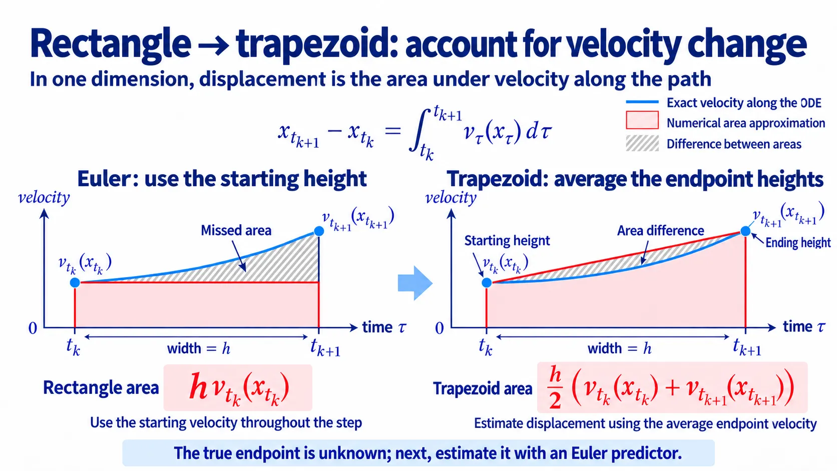
x_{t+h} \approx x_t+\frac h2\left(v_t(x_t)+v_{t+h}(x_{t+h})\right).

Rectangle and trapezoid approximations to the velocity integral.

Figure: replace a rectangle by a trapezoid. The blue curve is trajectory velocity; red is approximate displacement and gray indicates area discrepancy. This picture temporarily assumes both endpoint heights are known.

The true endpoint is unknown, so first predict it with Euler:

\widetilde x_{t+h}=x_t+h\,v_t(x_t).

Evaluate velocity there and correct the update using the average:

x_{t+h}^{\mathrm H} =x_t+\frac h2\left(v_t(x_t)+v_{t+h}(\widetilde x_{t+h})\right).

This Heun method uses an Euler predictor and a trapezoidal corrector. The predicted endpoint query prevents the initial arrow from determining the entire displacement alone.

Why does averaging recover the acceleration term?

For a sufficiently smooth field, velocity at the predicted endpoint expands as

v_{t+h}(\widetilde x_{t+h}) =v_t(x_t)+h\,a_t(x_t)+O(h^2).

The two arrows differ by approximately $ha_t$ . Substituting gives

\begin{aligned} x_{t+h}^{\mathrm H} &=x_t+\frac h2\left(v_t(x_t)+v_{t+h}(\widetilde x_{t+h})\right)\\ &=x_t+h\,v_t(x_t)+\frac{h^2}{2}a_t(x_t)+O(h^3). \end{aligned}

Heun recovers the quadratic Taylor term. Its local error is $O(h^3)$ and global error $O(h^2)$ , compared with Euler’s $O(h^2)$ local and $O(h)$ global errors:

\text{Euler global error}=O(h), \qquad \text{Heun global error}=O(h^2).

This correction is used in diffusion sampling by Karras and colleagues [1]. Heun generally costs 2 NFE per step. An $M$ -NFE budget therefore allows $M$ Euler steps but only $M/2$ Heun steps.

Equal step sizes may spend queries in the wrong places

On a nearly constant-velocity segment, repeated checks can be wasteful. Around rapid changes, sparse checks are inaccurate. We would like large steps in stable regions and small steps where needed.

We do not know these regions beforehand. Compare one full Euler step with two half steps:

\begin{aligned} x_{\mathrm{full}}&=x_t+h\,v_t(x_t),\\ x_{\mathrm{half}}&=x_t+\frac h2v_t(x_t),\\ x_{\mathrm{two}}&=x_{\mathrm{half}}+\frac h2v_{t+h/2}(x_{\mathrm{half}}). \end{aligned}

Taylor expansion shows

x_{\mathrm{two}}-x_{\mathrm{full}} =\frac{h^2}{4}a_t(x_t)+O(h^3).

Their discrepancy is not the true error, but supplies a local error signal. Accept when it falls within a chosen tolerance; otherwise reject the attempt and retry with a smaller step.

This is adaptive step size. Fixed-step Heun is not automatically adaptive, but its predictor and corrector already provide two approximations:

\left\|x_{t+h}^{\mathrm H}-\widetilde x_{t+h}\right\|

Their difference can drive a controller. Embedded Runge–Kutta methods similarly share queries between approximations of different orders; Dormand–Prince [2] is a standard example. Rejected attempts and error estimates still cost NFE, and different samples may require different grids.

Interactive demo. Euler and Heun use equal NFE budgets on a smooth rotating field, so Heun takes half as many steps. Adaptive mode uses predictor-corrector disagreement to place denser nodes where needed.

DiscussionQ1

With 20 NFE each, must second-order Heun beat first-order Euler?

Show the reasoning

No. Order describes the asymptotic rate as step size vanishes, not a universal ranking at every budget.

Euler can take 20 steps while Heun takes 10. Smooth trajectories and moderate higher-derivative constants often favor Heun, but coarse steps or large error constants can reduce that advantage.

Compare total NFE, error order, and the field’s smoothness together.

Integrate known structure exactly when possible

General solvers treat velocity as a black box. Gaussian-path diffusion instead offers a semilinear form:

\frac{\mathrm dx_t}{\mathrm dt} =A(t)x_t+B(t)\,\epsilon_\theta(x_t,t),

The schedule determines $A(t)$ and $B(t)$ ; only the neural term needs model calls. The exact update can be rewritten as

\begin{aligned} x_t &=e^{\int_s^t A(r)\,\mathrm dr}x_s\\ &\quad+\int_s^t e^{\int_\tau^t A(r)\,\mathrm dr} B(\tau)\,\epsilon_\theta(x_\tau,\tau) \,\mathrm d\tau. \end{aligned}

The linear evolution is analytic, leaving only the neural integral to approximate. DPM-Solver [3] uses this structure and a log-SNR time coordinate to build higher-order approximations.

DetailsDerive the exact update using an integrating factor

Define

m(t)=\exp\!\left(-\int_s^t A(r)\,\mathrm dr\right).

Multiply the ODE by this factor. The product rule cancels the linear term:

\frac{\mathrm d}{\mathrm dt}\bigl(m(t)x_t\bigr) =m(t)B(t)\epsilon_\theta(x_t,t).

Integrate and divide by the factor to obtain the displayed update. This is the integrating-factor or variation-of-constants formula.

This advantage requires an ODE with exploitable structure. An arbitrary Flow Matching field may instead call for a general solver such as Heun or adaptive Runge–Kutta.

An accurate solver still follows the field it receives

Refining a solver approaches the exact trajectory of the learned field. If that field is wrong, numerical accuracy does not restore the ideal probability path.

Modeling and numerical errors are separate. The solver methods improve the numerical contribution discussed in U3.1.

A solver controls how accurately we follow a given field, rather than whether that field is correct.

Check your understanding

References

Karras, T., Aittala, M., Aila, T., Laine, S. Elucidating the Design Space of Diffusion-Based Generative Models. NeurIPS 2022.
Dormand, J. R., Prince, P. J. A Family of Embedded Runge–Kutta Formulae. 1980.
Lu, C., et al. DPM-Solver: A Fast ODE Solver for Diffusion Probabilistic Model Sampling in Around 10 Steps. NeurIPS 2022.