After seeing corgis in snowy mountains, the user says, “These are all correct, but I prefer this lighting and composition. Could I have several different results?” They give us an aesthetic scoring program: input a finished image and receive a score.
Write a clean, finished image as x0 and its reward as R(x0). Higher scores better match this criterion. A reward can simply be an aesthetic score: it need not be a probability or differentiable. First specify how we want to sample; later, check the conditions for computing a direction. We have no noisy-image classifier for this preference, and the model has not learned it. Before changing the sampler, how should the score affect returned results?
Mugi: keep the favorite
MugiA corgi with a Shiba face
“If the program scores images, let us draw many and keep the highest-scoring one. When the user returns tomorrow, give them that same image?”
This uses the score and can find a high-scoring result. But the user also wanted several different results. Does keeping only the highest-scoring image express that request?
Nori: just draw more as before?
NoriA polar bear in an orca hat
“If we want to avoid returning the same image every time, sample as before. More draws will give different results.”
Nori preserves the original variation. But the user specifically preferred certain lighting and composition. If frequencies stay exactly the same, has this score affected the results?
Lumi: could we change the frequencies?
LumiA winged deer
“Could preferred photos appear more often without taking every chance away from other plausible photos? Across several draws, perhaps we would see the preferred style more often, but occasionally another composition.”
Lumi wants to change the proportions in which images are sampled. We want more than one highest-scoring image and more than the unchanged base proportions. What objective would express this idea?
Return the same favorite every time?
LumiA winged deer
Revisit the partners’ proposals
The user wants preferred results more often while retaining different plausible answers. Which approach better expresses both requirements?
It can find a high-scoring result, but repeating one image does not express the request for varied answers.
Making preferred results more frequent while retaining alternatives means choosing a new sampling distribution.
The original proportions retain variation, but the newly supplied scores have no effect.
What does the base contribute besides preference?
NoriA polar bear in an orca hat
“What if the scorer especially likes a bright white blob that is not a corgi? Do we want it to appear very often?”
We also want the original data to matter. Let pdata(x0) denote the base distribution: probabilities for discrete results, densities for continuous images. It tells us where the original data places more weight. It is not another aesthetic score, and it does not guarantee every high-density result is good.
To combine original weights and reward in one objective, start with logpdata(x0). Log turns multiplication into addition; we will see how this connects to KL between distributions. With finite rewards, reweighting alone cannot create results outside the original support.
Why use log probability? Think through model training
Switch briefly to training. We have independently drawn data x1,…,xn and change model parameters θ. Here i indexes data, not diffusion time. Likelihood and log-likelihood are
L(θ)=i=1∏npθ(xi),logL(θ)=i=1∑nlogpθ(xi).
Log is strictly increasing, so taking the log of the same likelihood leaves its maximizing parameters unchanged. Replacing products of small numbers with sums also helps computation. Dividing by fixed n preserves the maximizer too. Using the data average to estimate a population expectation gives Epdata[logpθ(x0)]. When the relevant quantities are defined,
The data distribution is fixed, so maximizing average log-likelihood minimizes KL in this direction. Training fixes the data and changes the model. We will instead fix the base and choose a new sampling distribution p. Keep these settings distinct.
Does “log preserves order” let us swap log and averaging? Suppose data probabilities for A,B are 0.9,0.1, while the model assigns a,1−a. Average probability is 0.9a+0.1(1−a), favoring a=1. Average log probability is
0.9loga+0.1log(1−a).
For 0<a<1, its derivative is 0.9/a−0.1/(1−a), zero at a=0.9. The second derivative is negative, so this is the maximum. It retains the rarer B. Taking a log after averaging and averaging logs optimize different objectives.
Is maximizing the average score enough?
MugiA corgi with a Shiba face
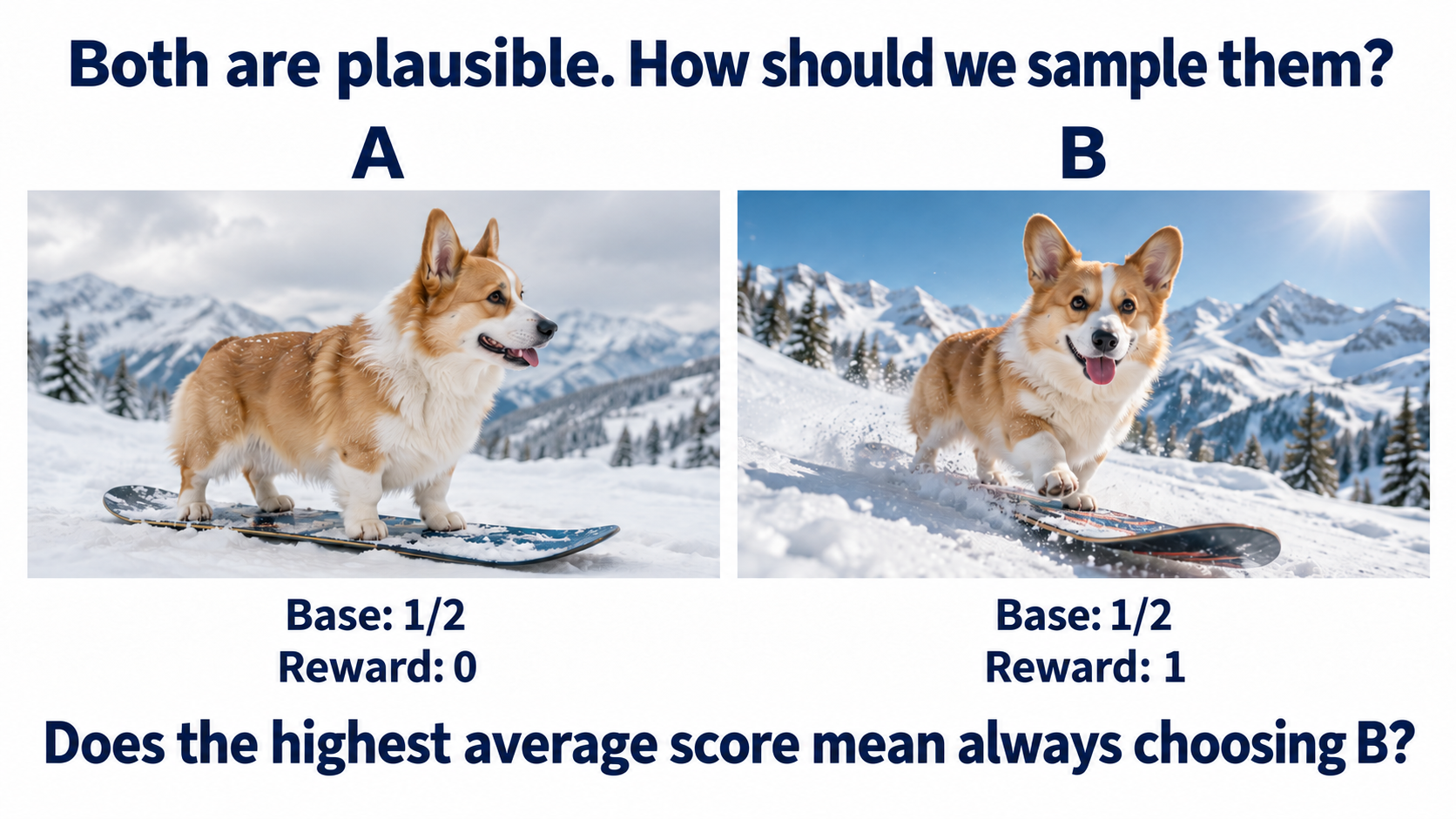
Both are plausible, with different lighting and poses. The example assumes the program prefers B. These probabilities and rewards are given toy values, not model measurements.
Select the image to enlarge
Simplify the possible results to A,B, originally equally likely, with rewards 0,1. The new distribution we choose, p, determines their future frequencies.
To favor reward while retaining the data’s influence, score each image by λR(x0)+logpdata(x0). Here λ>0 sets reward influence, and pdata is the base. These are two discrete results, each with probability 1/2; continuous images would use density.
Imagine repeatedly drawing from p and averaging this score. Will maximizing that average keep both photos, or choose B every time? Predict the result and explain why.
You can also think first, then read the explanation. Your writing stays on this page and disappears when you reload.
Add the two results’ contributions
MugiA corgi with a Shiba face
Both log base probabilities equal log(1/2)=−log2; only the reward differs. The new probabilities p(A),p(B) sum to 1, so the average score is
p(A)(−log2)+p(B)(λ−log2)=−log2+λp(B).
For any λ>0, assigning more probability to B raises the average, eventually returning B every time. Both images were plausible, but this average score never requires retaining the other answer.
Does this happen with more than two photos?
For finitely many candidates, write each fixed image score as
F(x0)=λR(x0)+logpdata(x0).
The average ∑x0p(x0)F(x0) cannot exceed the largest F. Assigning all mass to a highest-scoring candidate attains that value. Ties allow mixing among maximizers, but still do not encourage retaining other answers.
Continuous spaces need more care: an ordinary density may not attain a point-concentrated maximum; increasingly concentrated sequences might only approach it. The shared problem is averaging fixed per-image scores without separately measuring the new distribution’s concentration.
Which requirement is missing?
LumiA winged deer
The objective included both reward and log base probability, yet chose only B. Which original requirement still needs to enter?
The original objective only averages per-image scores; it does not measure excessive concentration of the whole distribution.
Reward already appears. Increasing it only favors B more here; it adds no requirement to retain alternatives.
The equal base probabilities already enter. What is missing is a measure of the new distribution’s concentration.
How can we express avoiding concentration?
LumiA winged deer
Entropy measures how spread out a distribution is: H(p)=−Ep[logp(x0)]. For our two photos, always choosing B gives 0, while equal probabilities give log2. Adding entropy makes spreading probability across answers contribute too:
Every expectation averages over x0 drawn from the new p. The scoring program, base, and λ stay fixed. We change the frequencies of results.
Can you write one log ratio?
LumiA winged deer
Expand entropy. All three terms average over the same p, so the objective value becomes
Ep[λR(x0)+logpdata(x0)−logp(x0)].
Use λR=logeλR and the product and quotient rules for log. How would you write the three terms inside as one log ratio? Start with its numerator and denominator.
You can also think first, then read the explanation. Your writing stays on this page and disappears when you reload.
The numerator offers a clue
LumiA winged deer
The added logs belong in the numerator, and the subtracted log in the denominator:
Ep[logp(x0)pdata(x0)eλR(x0)].
Look at the numerator: the original weight is multiplied by eλR(x0), giving higher-reward results larger multipliers. This resembles the desired reweighting, but is it already a probability distribution?
Can weights exceed 1?
NoriA polar bear in an orca hat
Keep base probabilities 1/2,1/2 and rewards 0,1. With λ=log3, the multipliers are 1,3, giving weights 1/2 for A and 3/2 for B. How should we interpret them?
Relative weights may exceed 1; probabilities may not. Normalization restores total mass to 1.
B’s value exceeds 1 and the total is 2, so these cannot yet be probabilities.
A relative weight exceeding 1 does not invalidate the multiplier. Normalize rather than clip it.
Restore total mass to 1
LumiA winged deer
Write the sum or integral of weights as ZR. Dividing by it defines a candidate distribution:
pR(x0)=ZRpdata(x0)eλR(x0).
For two photos, ZR is a sum; for continuous images, it integrates over all x0. Assume 0<ZR<∞ and that relevant expectations are defined. We still need to check that this candidate maximizes our objective.
Plot the base reweighted by reward
NoriA polar bear in an orca hat
Return from A/B outcomes to the continuous mixture from U7.0. Reward can favor the right or two regions. Inspect actual samples before proving why this candidate optimizes the objective.
Predict, then inspect the distribution
Starting from an equal mixture, does reward weighting change only the mode shares, or also shape and location within each mode?
A has λ = 0; B uses your reward and λ. Draw 1,000 samples from each one-dimensional numerical CDF.
The gray curve shows the original mixture. Running adds actual samples; a reference curve does not establish that it was sampled.
A: settings and observation
B: settings and observation
Fixed baseReference labelled after runningActual samplesA histogram outline
Explain using the plot and numbers
Weighting acts on every x0 and can change within-mode shape. The right reward favors the right mode and its tail; the symmetric reward can retain two peaks. A grid makes normalization and sampling possible here; images need the later sampling methods.
This explains the standard comparison. After changing controls or Python, use the settings and plots you actually ran.
Fixed base: ½N(-2,0.55²) + ½N(2,0.55²). Normalize p_base exp(λR) on [-6,6] with Δx = 0.025, invert the CDF, and sample uniformly within a bin. This is a numerical one-dimensional approximation, not a diffusion network.
Edit Python and run the experiment yourself
Change the parameters or the sampling rule. Python loads when you press Run and executes in your browser. Each run starts fresh; your edits are not saved.
The first opening imports the controls above; reopening preserves your edits. Settings are imported, not accumulated trained parameters or samples, so finite-sample plots need not match exactly.
The code implements this method and plots its distribution with Matplotlib. The first opening imports current controls; every run samples afresh. Change one parameter at the top. The native plot is not a record of edited Python output.
import math
import numpy as np
import matplotlib.pyplot as plt

# 1. SETTINGS -- change one, run again, and explain the plotted evidence.
strength = 2
reward_kind = "right"  # "right" or "two"
rng = np.random.default_rng(42)
sigma = 0.55
grid = np.linspace(-6, 6, 481)
dx = grid[1] - grid[0]

# 2. FIXED MODEL -- analytic functions, no network training in this cell.
def pdf(x, mu=0.0, var=1.0):
    return np.exp(-0.5 * (x-mu)**2 / var) / np.sqrt(2*np.pi*var)
def R(x):
    return x if reward_kind == "right" else -(np.abs(x)-2.5)**2
base = 0.5*pdf(grid, -2, sigma**2)+0.5*pdf(grid, 2, sigma**2)
target = base*np.exp(strength*R(grid))
target /= target.sum()*dx  # finite-grid quadrature reference
reference = target
reference_label = "Tilt reference (quadrature on [-6,6])"
extra_figure = None

# 3. GENERATION -- directly invert the finite-grid target CDF.
# This is possible in one dimension; it does not solve high-dimensional sampling.
cdf = np.cumsum(target*dx)
indices = np.searchsorted(cdf, rng.random(1000)).clip(0, len(grid)-1)
samples = grid[indices]+rng.uniform(-dx/2, dx/2, 1000)
print("Reference mass:", target.sum()*dx)
print("Target mean reward:", np.sum(target*R(grid))*dx)

# 4. PLOT AND CHECK -- the histogram is from the samples above.
fig, ax = plt.subplots(figsize=(8, 3.6))
ax.plot(grid, base, "--", color="gray", label="Original base")
ax.plot(grid, reference, ":", color="black", label=reference_label)
ax.hist(samples, bins=np.linspace(-6,6,49), weights=np.ones(len(samples))/(len(samples)*0.25), alpha=0.5, label="Actual generated samples")
ax.set(xlabel="clean x0", ylabel="density", xlim=(-6,6))
ax.legend(fontsize=8)
fig.tight_layout()
print("Outputs:", len(samples), "mean:", np.mean(samples), "right share:", np.mean(samples > 0))
print("Outside the plotted window:", np.sum(np.abs(samples)>6))
plt.show()
Package messages and warnings
Which part of the objective can change?
NoriA polar bear in an orca hat
Substitute pdataeλR=ZRpR into the log ratio. Separate the fixed logZR. The remaining average of log(pR/p) is negative KL:
KL measures the difference between these distributions. It is nonnegative and zero when they coincide. With base, reward, and λ fixed, which p maximizes the objective?
Subtracting a nonnegative quantity gives a maximum when that quantity is zero. We choose the new distribution, not the fixed scorer or base.
The objective subtracts KL. Larger KL lowers the value.
Fixed base, reward, and strength already determine Z_R. Choosing a new distribution does not change it.
Read the objective back into the situation
NoriA polar bear in an orca hat
“We now have new proportions that favor the user’s style while keeping the original distribution involved. Can ‘do not stray too far from the base’ appear directly in the objective?”
Yes. Entropy plus expected log base equals negative KL. Divide the objective by positive λ, which preserves its maximizer:
This KL direction differs from the earlier training example: now the expectation is over the p we choose.
A larger λ makes the penalty coefficient for departing from the base smaller. We allow preference more influence, but cannot conclude that images become more plausible.
What if I specify a maximum departure instead of a penalty?
We could maximize Ep[R] subject to DKL(p∥pdata)≤δ, where δ is the allowed departure.
With positive multiplier 1/λ, the Lagrangian is
Ep[R]−λ1[DKL(p∥pdata)−δ].
The final δ/λ is constant in p. For a fixed multiplier, this has the same optimizer as the KL-penalized objective. But arbitrary choices of δ,λ do not make the constrained and penalized problems equivalent.
For example, if pR has finite KL, choose δ=DKL(pR∥pdata). Optimality of pR implies that any feasible p satisfies
Thus pR also solves the constrained problem for this matched δ. This is the reason the two forms connect.
Can reweighting describe recovering an original from a blurry photo?
Suppose we observe y, such as an actually received blurry photo. Let p(y∣x0) describe how likely an original image is to produce this observation, and choose R(x0)=logp(y∣x0) and λ=1. Then
When 0<p(y)<∞, normalization gives the Bayes posterior p(x0∣y). Here y is an observation, unlike the desired condition “corgi.” It also differs from the base posterior given a sampling-time xt below. In this example, the observation enters as a log-likelihood reward.
Does preference learning for language models use this objective too?
Fix a prompt, view x0 as an answer, and let pref be the original answer distribution. A common preference objective is
pmax{Ep[R]−βDKL(p∥pref)},
Here β>0 controls retention of the reference. For this ideal distribution-level problem, λ=1/β and optimal relative weights are pref(x0)eR(x0)/β. This has the same structure as KL regularization in RLHF.
Actual language-model training usually updates policy parameters and faces capacity and optimization limits; some full objectives also include pretraining terms. This ideal optimal distribution is therefore not the exact outcome of every RLHF algorithm. Here we instead preserve generative parameters and try to change sampling.
Choose the return rule. What happens to the proportions?
MugiA corgi with a Shiba face
Return to the two plausible photos. A,B initially have equal probability and rewards 0,1. At λ=log3, the unnormalized weights are 1/2 and 3/2, totaling 2.
We have specified the desired proportions. Will your return rule actually produce them? Predict the share of B, then choose original sampling, reward maximization, or sampling the new weights. After one run, change the rule or the original proportions and compare.
What happened this time?
Compare your recent attempts
A worked example to compare
A and B initially have equal probability, with rewards 0 and 1. At λ = log 3, their weights are 1/2 and 3/2, giving target proportions A: 25%, B: 75%. Original sampling stays at 50/50; always maximizing reward returns only B. Sampling the new weights gives the target in this two-outcome example.
This is a discrete A/B model with direct weighted sampling. Reward maximization chooses from the support; it is separate from finite-candidate Best-of-N.
Edit Python and run the experiment yourself
Change the parameters or the sampling rule. Python loads when you press Run and executes in your browser. Each run starts fresh; your edits are not saved.
The first opening imports the controls above; reopening preserves your edits. Settings are imported, not accumulated trained parameters or samples, so finite-sample plots need not match exactly.
Package messages and warningsDoes the original data still matter?
NoriA polar bear in an orca hat
The new proportions use both base and reward. If the photos originally had unequal probabilities, multiply each original weight by its own reward multiplier rather than comparing rewards alone. Large multipliers can greatly amplify low-density regions; including a base does not guarantee every result is plausible.
We use ideal pdata to define the target. Actual generation uses a learned model, whose errors still matter. Now return to intermediate guidance: the scorer understands finished images, while we only have a noisy image.
Can a clean-image direction be moved straight to the middle?
LumiA winged deer
First assume base and reward are differentiable at the clean end. Take logs of pR=pdataeλR/ZR and differentiate with respect to the clean image:
“Original direction plus reward direction” looks much like U7.1. Indeed, R=logp(c∣x0) with λ=1 recovers the clean conditional score.
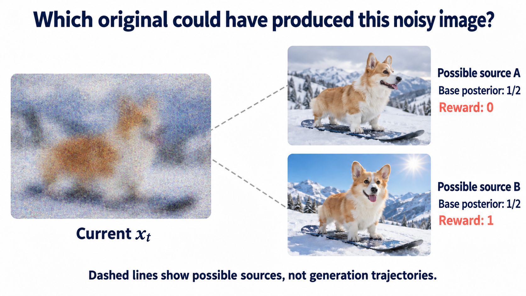
But we do not have finished x0, only xt. Does replacing subscript 0 with t let the same reward evaluate noise? First consider which clean photos could have produced this blurry image.
Where could this blurry image have come from?
NoriA polar bear in an orca hat
Fix the same xt. Equal posterior probabilities for A and B are a separate given assumption; equal base probabilities earlier do not imply it.
Select the image to enlarge
This xt could have come from A or B, whose rewards differ. What would you do first to bring clean-image reweighting to this state?
Each source has its own probability and reward weight. Uncertainty does not permit choosing just one source in advance.
The original model supplies base information; the new scorer has not entered the computation automatically. Ignoring it does not produce the new target.
Is the program receiving the input it understands?
NoriA polar bear in an orca hat
The aesthetic program was meant to judge composition and lighting in finished photos. Now it receives blurry noise. Even if it returns a number, that need not measure the intended request. Defining R on clean x0 does not make it valid on xt.
The same blurry outline could come from different photos with different rewards. Connecting the clean target to intermediate states requires handling those sources.
First go in the direction we know
LumiA winged deer
To find the noisy distribution corresponding to pR, draw a clean image from it and apply the original forward process. Use conditional density q(xt∣x0) for the noisy image given a clean source. Sum all sources’ contributions:
ptR(xt)=∫q(xt∣x0)⋅pR(x0)dx0.
We integrate over possible clean sources x0, holding the observed xt fixed. After substituting pR, we can rewrite the contributions as source probabilities given the current image.
Which factor can leave the integral?
LumiA winged deer
Substituting pR gives q(xt∣x0)pdata(x0) inside the integral. This is the base joint density, which Bayes’ rule also writes as
q(xt∣x0)pdata(x0)=pt(xt)p(x0∣xt).
When xt is fixed and we integrate over sources x0, which factor can move outside?
The integration variable is the clean source; base density at the fixed noisy image does not depend on it.
Different sources have different probabilities. This posterior supplies their weights and cannot leave the integral as a whole.
A and B have different reward multipliers. This factor depends on the clean source being integrated.
Which sources are being averaged?
NoriA polar bear in an orca hat
After taking out pt(xt), name the remaining average weight ht(xt):
Read the expectation as: “Given this xt, which clean photo could have produced it? Compute each source’s reward multiplier, then average by its probability.” This uses the base posterior p(x0∣xt), not a reward-modified posterior or an average over all data.
Average rewards, or average multipliers?
NoriA polar bear in an orca hat
The two sources are equally likely under the base posterior, with rewards 0,1. Again let λ=log3, giving multipliers 1,3. How should we compute ht for this xt?
h_t is the conditional average of reward multipliers, retaining both sources’ contributions.
Does preferring B mean it came from B?
MugiA corgi with a Shiba face
The scorer prefers B, but this xt need not have come from B. The base posterior still gives each source probability one half. Taking only the largest multiplier removes the other source’s contribution.
We need the average weight over possible sources, not the score of the best possible source.
Can averaging and exponentiation swap?
LumiA winged deer
Averaging rewards first gives 1/2 and then the exponential multiplier 3. Computing both multipliers first and averaging gives 2.
Exponentiation is nonlinear, so these orders need not agree. The definition of ht computes each source’s multiplier first, then takes the posterior average. Keep that order.
Mugi: what about estimating one clean image?
MugiA corgi with a Shiba face
“Including all possible sources sounds hard. We already have a denoiser. Could we denoise the current image, then give that to the aesthetic program?”
Recall xt=αˉtx0+σtϵ. Subtract predicted noise and divide out the signal scale:
x^0(xt,t)=αˉtxt−σtϵθ(xt,t).
Here αˉt>0 and σt=1−αˉt. Under ideal squared-error noise estimation, this equals the base posterior mean E[x0∣xt]; actual networks also have estimation error. It supplies a clean estimate, not a uniquely recovered true source.
Mugi proposes using eλR(x^0) instead of the needed ht. Which computation would this save, and which information might it remove?
Could one denoised estimate replace the average?
NoriA polar bear in an orca hat
Revisit the partners’ proposals
Recall x^0(xt,t): ideally it already averages possible sources. Mugi wants to score only this estimate, using eλR(x^0) instead of averaging individual source multipliers in ht. Does one mean estimate retain the average weight of all possible sources? Think about the order of averaging and nonlinear operations.
You can also think first, then read the explanation. Your writing stays on this page and disappears when you reload.
Calculate both orders and compare
MugiA corgi with a Shiba face
Temporarily replace high-dimensional images with numbers: A is x0=0 and B is x0=1, still equally likely given xt. Choose R(x0)=x0 and λ=log3, reproducing the previous rewards and multipliers.
Average the data first to get x^0=1/2, then evaluate its multiplier:
eλR(x^0)=e(log3)/2=3.
Computing source multipliers first and averaging gave ht=2. Even a linear reward leaves an outer exponential that makes the orders differ. Real image rewards are usually nonlinear too, so equality is even less justified.
Replacing the source average with a single denoised prediction is a plug-in approximation. It discards source uncertainty; the omitted quantity is more than a normalizing constant.
Plot possible sources, h_t, and plug-in
NoriA polar bear in an orca hat
Fix the noisy observation and inspect possible clean sources and their mean. A second plot shows h_t and plug-in across observations. See what uncertainty is lost before differentiating.
Predict, then inspect the distribution
For a fixed x_t = 0, how do possible clean sources change as noise increases? Does scoring their mean equal averaging their reward multipliers?
A uses noise time t = 0.08; B uses your t. The observation, reward, and λ stay fixed.
The gray curve shows the original mixture. Running adds actual samples; a reference curve does not establish that it was sampled.
A: settings and observation
B: settings and observation
Fixed baseReference labelled after runningActual samplesA histogram outline
Explain using the plot and numbers
The posterior describes possible clean sources. h_t averages their exponential reward multipliers; plug-in scores the mean location. A two-mode posterior can have a mean in a low-density gap. Nonlinearity makes the orders differ. The lower curves are weight functions, not densities or a claimed generated distribution.
This explains the standard comparison. After changing controls or Python, use the settings and plots you actually ran.
Sample 1,000 possible sources from the analytic Gaussian-mixture Bayes posterior. h_t uses analytic Gaussian integrals; plug-in uses the analytic posterior mean. This is the base posterior of a fixed noisy observation, not a reward-tilted posterior.
Edit Python and run the experiment yourself
Change the parameters or the sampling rule. Python loads when you press Run and executes in your browser. Each run starts fresh; your edits are not saved.
The first opening imports the controls above; reopening preserves your edits. Settings are imported, not accumulated trained parameters or samples, so finite-sample plots need not match exactly.
The code implements this method and plots its distribution with Matplotlib. The first opening imports current controls; every run samples afresh. Change one parameter at the top. The native plot is not a record of edited Python output.
import math
import numpy as np
import matplotlib.pyplot as plt

# 1. SETTINGS -- change one, run again, and explain the plotted evidence.
strength = 2
noise_time = 0.35
observed_x = 0
reward_kind = "two"  # "right" or "two"
rng = np.random.default_rng(42)
sigma = 0.55
grid = np.linspace(-6, 6, 481)
dx = grid[1] - grid[0]

# 2. FIXED MODEL -- analytic functions, no network training in this cell.
def pdf(x, mu=0.0, var=1.0):
    return np.exp(-0.5 * (x-mu)**2 / var) / np.sqrt(2*np.pi*var)
def Phi(x):
    return 0.5 * (1 + np.vectorize(math.erf)(np.asarray(x) / np.sqrt(2)))
def R(x):
    return x if reward_kind == "right" else -(np.abs(x)-2.5)**2
def moments(t):
    a = np.exp(-8*t)
    return np.sqrt(a), a*sigma**2 + 1-a
def sigmoid(v):
    return np.exp(-np.logaddexp(0, -v))
def post_params(x, t):
    signal, var = moments(t)
    right = sigmoid(4*signal*x/var)
    gain = signal*sigma**2/var
    left_mu = -2 + gain*(x + 2*signal)
    right_mu = 2 + gain*(x - 2*signal)
    variance = sigma**2*(1-np.exp(-8*t))/var
    return right, left_mu, right_mu, variance
def posterior_mean(x, t):
    w, m0, m1, v = post_params(x, t)
    return (1-w)*m0+w*m1
def h(x, t):
    if t == 0:
        return np.exp(strength*R(x))
    w, m0, m1, v = post_params(x, t)
    if reward_kind == "right":
        return (1-w)*np.exp(strength*m0+0.5*strength**2*v)+w*np.exp(strength*m1+0.5*strength**2*v)
    d = 1+2*strength*v
    def component(mu):
        result = 0.0
        for side in [-1, 1]:
            center = (mu+2*strength*v*side*2.5)/d
            factor = np.exp(-strength*(mu-side*2.5)**2/d)/np.sqrt(d)
            result += factor*Phi(side*center/np.sqrt(v/d))
        return result
    return (1-w)*component(m0)+w*component(m1)
base = 0.5*pdf(grid, -2, sigma**2)+0.5*pdf(grid, 2, sigma**2)
target = base*np.exp(strength*R(grid))
target /= target.sum()*dx  # finite-grid quadrature reference
reference = target
reference_label = "Tilt reference (quadrature on [-6,6])"
extra_figure = None

# 3. POSTERIOR -- sample possible clean sources of this fixed noisy observation.
w, m0, m1, v = post_params(observed_x, noise_time)
samples = np.where(rng.random(1000) < w, m1, m0)+np.sqrt(v)*rng.normal(size=1000)
reference = (1-w)*pdf(grid, m0, v)+w*pdf(grid, m1, v)
reference_label = "Base posterior p(x0 | xt)"
mean = posterior_mean(observed_x, noise_time)
exact = h(observed_x, noise_time)
plugin = np.exp(strength*R(mean))
print("Posterior mean:", mean, "h_t:", exact, "plug-in:", plugin)
extra_figure, ax = plt.subplots(figsize=(8, 3.2))
ax.plot(grid, h(grid, noise_time), label="h_t: average the reward MULTIPLIERS")
ax.plot(grid, np.exp(strength*R(posterior_mean(grid, noise_time))), label="plug-in: score the posterior MEAN")
ax.axvline(observed_x, color="gray", linestyle=":")
ax.set(xlabel="noisy observation x_t", ylabel="weight (not density)")
ax.legend(fontsize=8)
extra_figure.tight_layout()

# 4. PLOT AND CHECK -- the histogram is from the samples above.
fig, ax = plt.subplots(figsize=(8, 3.6))
ax.plot(grid, base, "--", color="gray", label="Original base")
ax.plot(grid, reference, ":", color="black", label=reference_label)
ax.hist(samples, bins=np.linspace(-6,6,49), weights=np.ones(len(samples))/(len(samples)*0.25), alpha=0.5, label="Actual generated samples")
ax.set(xlabel="clean x0", ylabel="density", xlim=(-6,6))
ax.legend(fontsize=8)
fig.tight_layout()
print("Outputs:", len(samples), "mean:", np.mean(samples), "right share:", np.mean(samples > 0))
print("Outside the plotted window:", np.sum(np.abs(samples)>6))
plt.show()
Package messages and warnings
How do weights give a direction?
LumiA winged deer
We have ptR=ptht/ZR. Follow U7.1: take logs, then differentiate with respect to the current image xt.
ZR does not change with the image, and the base term gives the original score. Which term supplies the extra direction this time? Try writing the new target’s score.
You can also think first, then read the explanation. Your writing stays on this page and disappears when you reload.
Differentiate the posterior-average weight
LumiA winged deer
Termwise differentiation gives
∇xtlogptR(xt)=st(xt)+∇xtloght(xt).
The extra direction is the log-gradient of ht: how the average weight of compatible sources changes with the current image. Exact ht is hard to compute, so a common approach replaces it with the plug-in estimate.
Which input are we differentiating now?
NoriA polar bear in an orca hat
Assume reward and denoised prediction are differentiable. We use R(x^0(xt,t)) for suggestions while keeping both networks fixed. Which calculation gives a direction for the current image?
Input gradients can pass through a fixed network. Fixed parameters do not make the output’s input derivative zero.
That changes the generative model, violating the fixed-parameter constraint.
Holding the denoised prediction constant removes its dependence on the current image. Its derivative with respect to the current image is also needed.
This step is an approximation
NoriA polar bear in an orca hat
The plug-in log is λR(x^0), so the extra direction is approximated by
∇xtloght(xt)≈λ∇xtR(x^0(xt,t)).
Write out the whole dependency using the chain rule:
∇xtR(x^0(xt,t))=(∂xt∂x^0)⊤∇x0R(x^0).
The reward gradient describes changes to the clean estimate that increase its score. The Jacobian ∂x^0/∂xt describes how that estimate changes with the current noisy image. Their product converts the direction back to the xt we can modify. Fixed θ still allows this input gradient.
Our example already showed unequal weights, so this approximation cannot simply be called exact tilting. Even exact scores need the correct initial noisy distribution and reverse dynamics for actual sampling. Network estimation, finite noise, and a finite-step sampler add approximations to check.
Why check even the initial noise distribution?
The same reweighting relation holds at starting time T:
pTR(xT)=ZRpT(xT)hT(xT).
If the forward process has completely forgotten the clean source, xT and x0 are independent, so
hT(xT)=Epdata[eλR(x0)]=ZR.
Then pTR=pT, allowing the same base start. Finite noise need not achieve full independence. Even highly accurate scores do not establish exact sampling when started from a mismatched distribution.
Which approximations do practical methods address?
A common practical route converts noisy images into denoised predictions, then uses an external differentiable request for a direction. Universal Guidance discusses such use. Separating it from the exact posterior average shows where source uncertainty was omitted.
For example, Calibrated Test-Time Guidance analyzes how common approximations bias Bayesian posterior sampling and proposes a consistent estimator under its conditions. Are We Really Tilting? separates mode selection from excessive reward pursuit within modes in Gaussian and mixture examples, and studies reward damping. Read each result with its assumptions; do not extend it to arbitrary rewards and samplers.
Methods can improve posterior approximations, adjust guidance strength, or constrain updates. But a higher average reward checks only one quantity. Excessive preference strength may suppress plausible lower-scoring modes. Assess reward, plausibility, diversity, and whether the defined target is actually sampled separately.
Does a higher score establish the right proportions?
NoriA polar bear in an orca hat
A batch generated with plug-in guidance has higher average reward than before. Does this number alone prove that the sampler draws from our defined pR?
Explain the difference using your plots
NoriA polar bear in an orca hat
Choose a reward and λ from your experiment. Use the target curve, generated histogram, and a posterior-mean or h_t value to explain the evidence needed for higher reward, a correctly defined weight, and actual target sampling.
You can also think first, then read the explanation. Your writing stays on this page and disappears when you reload.
Check each kind of evidence
NoriA polar bear in an orca hat
Mean reward addresses the scoring metric. Normalization and derivation define the target. Sampling requires comparing proportions, shape, and missing regions. A one-dimensional finite histogram fluctuates and does not provide the same exact check for real images.
Finally, try different base proportions
LumiA winged deer
Now let base probabilities of A,B be 3/4,1/4, keeping rewards 0,1 and λ=log3, hence multipliers 1,3. Which reweighted proportions meet the target?
A is originally three times as common, while B has three times the reward multiplier. The products are equal.
That ignores the original probabilities and uses only multipliers 1:3. The base proportions have changed.
That retains the original proportions without applying B’s multiplier of three.
What if the program only returns scores?
MugiA corgi with a Shiba face
For our two plausible photos, we wanted preferred results more often while retaining alternatives and the base’s influence. Reward tilting defines new proportions. Intermediate guidance must consider compatible clean sources. Replacing their average with one denoised estimate eases computation, but remains an approximation.
If the program only returns scores and cannot be differentiated, we cannot directly compute that direction. Could we generate candidates and change returned proportions by comparing scores alone? Continue in U7.3, where we will examine candidate counts and computation cost.