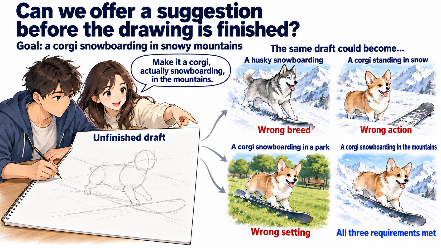
Consider a concrete task. Our model is already trained, and we want a corgi snowboarding in snowy mountains. Even if it accepts text, does supplying those words guarantee the image we want?
Perhaps the dog is snowboarding in the mountains but turns out to be a husky. Perhaps the corgi and mountains are right, but the dog merely stands in the snow. We want to keep the model’s parameters and offer clues while the image is still unfinished.
The same sketch can develop into different results. For now, we only address “is it a corgi?” Snowy mountains and snowboarding remain separate requirements.
Select the image to enlarge
Lumi: ask a helper that understands drafts
LumiA winged deer
“If the dog’s legs keep getting longer halfway through drawing, could a friend check how much this image still resembles a corgi?”
Lumi wants a model that recognizes breeds in noisy images. Show it the current image, then find small changes that increase its probability of calling the image a corgi. This is classifier guidance: the classifier provides the judgment, and guidance connects that judgment to generation.
Mugi: could the model answer twice?
MugiA corgi with a Shiba face
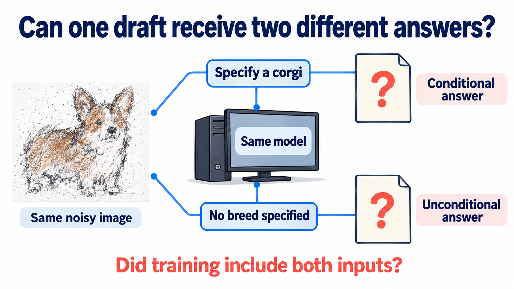
“If the model already reads descriptions, could we ask about the same draft twice? Once say ‘draw a corgi,’ and once leave the breed unspecified. How do the answers differ?”
Mugi wants to compare the same generative model’s predictions with and without a description, then strengthen what the request adds. This is classifier-free guidance (CFG). It needs no separate classifier, but the model must actually have learned both kinds of input.
Nori: check what our tools can answer
NoriA polar bear in an orca hat
“We can describe both ideas. But if the helper has only seen clean photos, can it understand all this noise? If the model always received a description, how will it answer without one?”
Nori wants to check what was learned before generation. At each step, ask: Whose answer do we need now? Has it learned to handle this input? Then examine how Lumi’s and Mugi’s proposals connect to the image in front of us.
What should the helper see now?
LumiA winged deer
Revisit the partners’ proposals
We want a suggestion at the current step, rather than waiting to select a finished image. What should we give the helper first?
An intermediate adjustment must use the current state. The helper must understand noisy images before its judgment is useful at this step.
A finished photo is useful for final selection, but it does not exist yet. Intermediate guidance must use an input available now.
The fraction of corgis in the dataset does not describe this particular image. The judgment needs to inspect it.
Can we find clues in the draft?
NoriA polar bear in an orca hat
Imagine drawing a few blurry lines. The animal looks vaguely like a dog, but its breed is unclear. A friend suggests, “Would shorter legs make it look more like a corgi?” We can try changing the draft rather than finishing the whole image and starting over.
In diffusion, our actual input is a noisy image xt. The desired “corgi” is the condition c. Keep U1’s time convention: larger t means more noise, and sampling moves toward clean images at t=0. The noisy image is formed as
xt=αˉtx0+σtϵ.
Here x0 is the original clean photo, αˉt is the retained signal fraction, ϵ∼N(0,I) is added noise, and σt=1−αˉt sets its amplitude. We therefore find a judgment model trained at different noise levels and ask it a class question.
Which question is it answering?
LumiA winged deer
Show the helper xt and ask: “How likely is this noisy image to have come from a corgi photo?” Which quantity answers that question?
The observed image is on the conditioning side; the class we want to infer is on the other side.
Changing the image leaves the dataset’s corgi fraction unchanged. This quantity has not inspected the image.
Which comes first: image or breed?
NoriA polar bear in an orca hat
pt(xt∣c) means “specify corgis, then describe their distribution after adding noise.” By contrast, pt(c∣xt) means “see this image, then infer its class.” We gave the helper an image, so it directly answers the latter.
We want to generate the images described by the former. These quantities are related, but we need to derive that connection rather than swap the notation.
How does judgment connect to generation?
LumiA winged deer
Imagine selecting the corgi photos in the data, then adding noise with the original forward process. Their noisy density is pt(xt∣c), the distribution we want for this breed.
Yes, it is time for Bayes’ rule again:
pt(xt∣c)=p(c)pt(xt)pt(c∣xt).
The base pt(xt) includes all kinds of images. Multiplying by the probability of “came from a corgi” gives relatively more weight to images likely to be corgis. The denominator p(c) restores total mass to 1. The helper’s judgment now connects to the images we want to generate.
How does the starting distribution enter this relationship?
The pt(xt∣c) above is a whole family of noisy distributions: draw clean x0 from the specified breed, then apply the same noising rule. Larger t usually obscures more of the original image.
If αˉT is very small, conditional xT is also close to a standard Gaussian, so reverse sampling can start from approximate noise. Finite noising need not erase all breed information, however: pT(xT∣c) is not necessarily exactly Gaussian. The score identity, network estimation, starting approximation, and discretized sampler are separate steps.
If only the image changes, what changes with it?
LumiA winged deer
Fix the noise level, the corgi request, and the original data. Change only the image slightly. Classify the three quantities in Bayes’ rule by their dependence on that image.
Image-dependent · Base density The current image’s base density.
Image-dependent · Class probability The probability of a corgi after seeing the image.
Fixed here · Class fraction The fraction of corgis in the data.
Turn density into a direction for change
LumiA winged deer
Having a density is not enough; we need a direction in which to change the image. Recall that a score differentiates log density with respect to the image. Taking logs first turns Bayes’ multiplication into addition:
logpt(xt∣c)=logpt(xt)+logpt(c∣xt)−logp(c).
Now differentiate with respect to xt. The original-data term gives the base score; the fixed term has zero derivative. Which term contributes the extra direction for corgis? Try writing its gradient.
You can also think first, then read the explanation. Your writing stays on this page and disappears when you reload.
The extra direction from specifying a breed
LumiA winged deer
Denote the conditional score by st(xt∣c) and the base score by st(xt). Termwise differentiation gives
st(xt∣c)=st(xt)+∇xtlogpt(c∣xt).
The last term points toward the fastest local increase in the log-probability of “came from a corgi” as we change xt. The directions add because Bayes’ product becomes a sum after taking logs.
This is a relationship between exact densities and scores. In practice, networks estimate them for a reverse-time sampler. The score itself is not the distance to move the image. Differentiating away p(c) also does not mean we have computed its value.
A one-dimensional draft we can actually generate
NoriA polar bear in an orca hat
Reuse U7.0: pbase=21N(−2,0.552)+21N(2,0.552), with left/right labels c=0,1. Choosing a class stands in for choosing corgis; the horizontal axis is a scalar datum, not a generated dog photograph.
This model has analytic noisy densities, class probabilities, and scores. First run an actual reverse sampler with ideal fixed tools. Each route then fully checks how real networks learn the required answers and how to express the result as noise prediction.
Explore a complete method, then return for the next
Choose the order. Each route includes prediction, actual sampling plots, full derivations, and limitations. Only returning from its final step marks it fully explored. You may return early and resume later.
Ask a noisy classifier for a direction
Run first: which samples does classifier guidance change?
LumiA winged deer
Use the ideal noisy classifier defined above. Compare the sampled A/B histograms, then inspect the directions and a sampler step at the same x_t.
Predict, then inspect the distribution
With the model fixed, what changes from no guidance to w = 1? Is the classifier gradient itself the sampler update?
A uses w = 0; B uses your chosen w. Both use identical initial noise and random seeds.
The gray curve shows the original mixture. Running adds actual samples; a reference curve does not establish that it was sampled.
A: settings and observation
B: settings and observation
Fixed baseReference labelled after runningActual samplesA histogram outline
Explain using the plot and numbers
The classifier supplies the input derivative of log class probability. The combined score goes into a reverse SDE whose update also includes drift, step size, and random noise. These are analytic functions, not trained networks. At w = 1 the endpoint approximates the conditional distribution, with finite-time and discretization error.
This explains the standard comparison. After changing controls or Python, use the settings and plots you actually ran.
VP: alpha_bar(t) = exp(-8t). Start from the exact base p_1 and use Euler–Maruyama toward t = 0: Δx = (4x + 8s̃)Δt + sqrt(8Δt)ξ. The dotted curve is a conditional reference at w = 1, not an exact endpoint target for w > 1.
Edit Python and run the experiment yourself
Change the parameters or the sampling rule. Python loads when you press Run and executes in your browser. Each run starts fresh; your edits are not saved.
The first opening imports the controls above; reopening preserves your edits. Settings are imported, not accumulated trained parameters or samples, so finite-sample plots need not match exactly.
The code implements this method and plots its distribution with Matplotlib. The first opening imports current controls; every run samples afresh. Change one parameter at the top. The native plot is not a record of edited Python output.
import math
import numpy as np
import matplotlib.pyplot as plt

# 1. SETTINGS -- change one, run again, and explain the plotted evidence.
strength = 1
condition = 1  # 0 = left, 1 = right
noise_time = 0.35
observed_x = 0
steps = 600
rng = np.random.default_rng(42)
sigma = 0.55
grid = np.linspace(-6, 6, 481)
dx = grid[1] - grid[0]

# 2. FIXED MODEL -- analytic functions, no network training in this cell.
def pdf(x, mu=0.0, var=1.0):
    return np.exp(-0.5 * (x-mu)**2 / var) / np.sqrt(2*np.pi*var)
def moments(t):
    a = np.exp(-8*t)
    return np.sqrt(a), a*sigma**2 + 1-a
def sample_base(size, t=0.0):
    signal, var = moments(t)
    mu = np.where(rng.random(size) < 0.5, -2.0, 2.0)
    return signal*mu + np.sqrt(var)*rng.normal(size=size)
def sigmoid(v):
    return np.exp(-np.logaddexp(0, -v))
base = 0.5*pdf(grid, -2, sigma**2)+0.5*pdf(grid, 2, sigma**2)
reference = base.copy()
reference_label = "Conditional reference at w=1"
extra_figure = None

# 3. GENERATION -- reverse VP SDE, Euler-Maruyama; beta = 8.
def base_score(x, t):
    signal, var = moments(t)
    right = sigmoid(4*signal*x/var)
    return (2*signal*(2*right-1)-x)/var
def conditional_score(x, t):
    signal, var = moments(t)
    return ((2 if condition else -2)*signal-x)/var
def classifier_log_gradient(x, t):
    signal, var = moments(t)
    right = sigmoid(4*signal*x/var)
    return 4*signal/var*((1-right) if condition else -right)
def guided(x, t):
    return base_score(x, t)+strength*classifier_log_gradient(x, t)
samples = sample_base(1000, 1.0)
dt = 1/steps
for k in range(steps, 0, -1):
    t = k*dt
    samples += (4*samples+8*guided(samples, t))*dt + np.sqrt(8*dt)*rng.normal(size=samples.size)
reference = pdf(grid, 2 if condition else -2, sigma**2)
reference_label = "Conditional reference at w=1 (not an exact w>1 target)"
print("Fixed analytic scores; finite-time and Euler error remain.")
print("Reverse steps:", steps, "sampler updates:", 1000*steps)
print("Signals per update: base score + classifier input gradient")
print("At x_t, base / conditional / classifier gradient:", base_score(observed_x, noise_time), conditional_score(observed_x, noise_time), classifier_log_gradient(observed_x, noise_time))

# 4. PLOT AND CHECK -- the histogram is from the samples above.
fig, ax = plt.subplots(figsize=(8, 3.6))
ax.plot(grid, base, "--", color="gray", label="Original base")
ax.plot(grid, reference, ":", color="black", label=reference_label)
ax.hist(samples, bins=np.linspace(-6,6,49), weights=np.ones(len(samples))/(len(samples)*0.25), alpha=0.5, label="Actual generated samples")
ax.set(xlabel="clean x0", ylabel="density", xlim=(-6,6))
ax.legend(fontsize=8)
fig.tight_layout()
print("Outputs:", len(samples), "mean:", np.mean(samples), "right share:", np.mean(samples > 0))
print("Outside the plotted window:", np.sum(np.abs(samples)>6))
plt.show()
Package messages and warnings
What do we want to change?
NoriA polar bear in an orca hat
Write the noisy classifier as pϕ(c∣xt,t), with parameters ϕ; the generative parameters remain θ. We want to keep the helper’s judgment rule and change the image it sees to increase the class log-probability. With respect to what should we differentiate?
An input gradient describes how the judgment varies with the input; it is not a network-parameter update direction.
Updating generative parameters would teach the model this preference again. We want clues for modifying the current image.
If the judgment rule changes, did the image change?
NoriA polar bear in an orca hat
Imagine keeping the image and changing only classifier parameters ϕ. Its judgment might change, but did the dog become a corgi? We want to preserve the judgment rule and change xt instead.
We therefore need ∇xtlogpϕ(c∣xt,t). Backpropagation can compute input gradients too. Computing a derivative and updating parameters are different operations.
Which helper is prepared for this image?
LumiA winged deer
Two candidates are available. A learned breeds only from clean photos; B learned the same task at different noise levels. Generation still contains noise. Which has at least the training preparation we need?
Noise level changes what the image reveals. The helper needs to learn class judgments on these inputs.
Accuracy on clean photos does not guarantee understanding of noisy inputs. Check what the helper actually practiced.
They see different inputs. Equal network size or the same name cannot replace training on the relevant inputs.
How should this helper practice?
LumiA winged deer
“There are many levels of blur along the way. Let us add different amounts of noise to a breed-labeled photo. Even as the dog becomes hard to recognize, we still know its original breed, right?”
Let ϕ denote the helper’s parameters. Draw (x0,c), a noise level t, and Gaussian noise ϵ, then form xt with the same noising rule. Ask it to assign probability to the correct breed. Its training loss is
Lcls(ϕ)=E(x0,c),t,ϵ[−logpϕ(c∣xt,t)].
Higher probability for the correct breed means smaller negative log-probability. This is the noisy classifier’s training exercise: directly noise training photos, without waiting for the generative model to draw them. At high noise, the photo may genuinely be unrecognizable, so a reasonable answer may be uncertain.
Training changes ϕ using ∇ϕLcls. To help change an image now, fix ϕ and use ∇xtlogpϕ(c∣xt,t). Both are gradients, but the object to be changed differs.
Put the needed directions together
LumiA winged deer
Estimate the base score with the trained model, then add the helper’s input gradient:
sθ(xt,t,c)=sθ(xt,t)+w∇xtlogpϕ(c∣xt,t).
Here w sets the suggestion’s strength. Starting from an unconditional base, w=0 retains the base; if both estimates are exact, w=1 gives the conditional score derived above. In practice, the reverse sampler uses this combined score to determine the next image update. This is Lumi’s classifier-guidance proposal.
What if the generative model already uses a condition?
We started from an unconditional base. Adding classifier guidance to an already conditional score is extra strengthening beyond the original request; an extra coefficient of 0 retains the conditional prediction. The two starting points cannot both call w=1 “no strengthening.” First identify the base answer, then inspect the extra term’s coefficient.
What if the network predicts noise?
LumiA winged deer
U1’s network usually outputs ϵθ. At a noisy time, with noise amplitude σt=1−αˉt>0, its score representation is
sθ(xt,t)=−σtϵθ(xt,t).
First consider classifier guidance: add w times the classifier’s input gradient to an unconditional base score. What happens to the extra term’s sign and scale in noise-prediction form? Multiply the whole score equation by −σt.
You can also think first, then read the explanation. Your writing stays on this page and disappears when you reload.
Both the minus sign and σt come from the conversion. Here classifier guidance starts from an unconditional base, so w=0 means no guidance. CFG instead starts from a conditional answer and uses w=1 as its baseline.
Does an accurate judgment imply an accurate direction?
NoriA polar bear in an orca hat
We use the gradient of probability as the image changes. Two terrains can have similar heights but different local slopes. Likewise, accurate class probabilities do not automatically imply accurate input gradients.
The generative model in this approach need not accept c; a separate noisy classifier supplies the request. Now suppose our available tool differs: if the generative model already learned the condition, could its own answers reveal this direction?
What else should we check about the helper?
Classification accuracy checks answers. Guidance also uses local changes around an image, so ask whether tiny input perturbations cause stable judgments. A classifier may change its answer sharply under a small perturbation; clean-image accuracy alone does not establish the quality of intermediate input gradients. This motivates examining the direction, without claiming that stability guarantees successful generation. Kawar, Ganz, and Elad study robust classifiers for guidance.
From the distribution to the complete formula
NoriA polar bear in an orca hat
You generated samples with a fixed model, distinguished input derivatives from parameter updates, and read the noisy-classifier loss, score combination, noise conversion, and limitations. Return to explore the other signal source.
Compare two predictions of the same model
Which two answers should we compare?
MugiA corgi with a Shiba face
For now, suppose the available model can also answer without a breed specification. Ask about the same xt at the same t twice, with and without “corgi.” How can we isolate what the request adds?
Bayes gave conditional = base + extra direction. Subtract the base from both sides; no need to repeat the full derivation.
Averaging retains the shared base. We want to isolate the effect of specifying the breed.
Did we count the shared part twice?
NoriA polar bear in an orca hat
We derived conditional score = base score + the condition’s extra direction. Adding the entire conditional score to the base counts that base a second time.
To retain only the condition’s effect, subtract the shared base. We compare two answers for the same image, not two finished images.
Which term did we subtract?
MugiA corgi with a Shiba face
Rearrange the exact score identity:
∇xtlogpt(c∣xt)=st(xt∣c)−st(xt).
Subtracting the original direction from the requested direction leaves exactly what the condition adds. Mugi proposes estimating the two terms on the right with the generative model, then subtracting. Use the same image at the same time to compare requests; subtracting two generated images cannot replace this operation.
Run first: how do two predictions change generation?
MugiA corgi with a Shiba face
Use this toy’s analytic conditional and unconditional scores at the same x_t and t. Then check the training prerequisites for real networks to supply them.
Predict, then inspect the distribution
Ask the same x_t with and without the condition. What changes within the selected mode when w increases from 1?
A retains the conditional prediction (w = 1); B uses your w. The condition, step count, and random seed stay fixed.
The gray curve shows the original mixture. Running adds actual samples; a reference curve does not establish that it was sampled.
A: settings and observation
B: settings and observation
Fixed baseReference labelled after runningActual samplesA histogram outline
Explain using the plot and numbers
CFG changes the combination of two predictions at one input. This toy uses ideal analytic predictions. w = 1 retains the conditional prediction. Larger w changes generation, but the amount of change depends on the data and condition; narrowing is not guaranteed. Ideal classifier guidance and CFG agree with the same w and sampler; real networks have different prerequisites and errors.
This explains the standard comparison. After changing controls or Python, use the settings and plots you actually ran.
The same VP sampler and fixed parameters use s̃ = s_c + (w−1)(s_c−s_empty). Analytic predictions isolate the combination. The following training derivation still checks conditioning dropout; an unprepared network is not assumed to answer empty inputs.
Edit Python and run the experiment yourself
Change the parameters or the sampling rule. Python loads when you press Run and executes in your browser. Each run starts fresh; your edits are not saved.
The first opening imports the controls above; reopening preserves your edits. Settings are imported, not accumulated trained parameters or samples, so finite-sample plots need not match exactly.
The code implements this method and plots its distribution with Matplotlib. The first opening imports current controls; every run samples afresh. Change one parameter at the top. The native plot is not a record of edited Python output.
import math
import numpy as np
import matplotlib.pyplot as plt

# 1. SETTINGS -- change one, run again, and explain the plotted evidence.
strength = 3
condition = 1  # 0 = left, 1 = right
noise_time = 0.35
observed_x = 0
steps = 600
rng = np.random.default_rng(42)
sigma = 0.55
grid = np.linspace(-6, 6, 481)
dx = grid[1] - grid[0]

# 2. FIXED MODEL -- analytic functions, no network training in this cell.
def pdf(x, mu=0.0, var=1.0):
    return np.exp(-0.5 * (x-mu)**2 / var) / np.sqrt(2*np.pi*var)
def moments(t):
    a = np.exp(-8*t)
    return np.sqrt(a), a*sigma**2 + 1-a
def sample_base(size, t=0.0):
    signal, var = moments(t)
    mu = np.where(rng.random(size) < 0.5, -2.0, 2.0)
    return signal*mu + np.sqrt(var)*rng.normal(size=size)
def sigmoid(v):
    return np.exp(-np.logaddexp(0, -v))
base = 0.5*pdf(grid, -2, sigma**2)+0.5*pdf(grid, 2, sigma**2)
reference = base.copy()
reference_label = "Conditional reference at w=1"
extra_figure = None

# 3. GENERATION -- reverse VP SDE, Euler-Maruyama; beta = 8.
def base_score(x, t):
    signal, var = moments(t)
    right = sigmoid(4*signal*x/var)
    return (2*signal*(2*right-1)-x)/var
def conditional_score(x, t):
    signal, var = moments(t)
    return ((2 if condition else -2)*signal-x)/var
def classifier_log_gradient(x, t):
    signal, var = moments(t)
    right = sigmoid(4*signal*x/var)
    return 4*signal/var*((1-right) if condition else -right)
def guided(x, t):
    sc, su = conditional_score(x, t), base_score(x, t)
    return sc+(strength-1)*(sc-su)
samples = sample_base(1000, 1.0)
dt = 1/steps
for k in range(steps, 0, -1):
    t = k*dt
    samples += (4*samples+8*guided(samples, t))*dt + np.sqrt(8*dt)*rng.normal(size=samples.size)
reference = pdf(grid, 2 if condition else -2, sigma**2)
reference_label = "Conditional reference at w=1 (not an exact w>1 target)"
print("Fixed analytic scores; finite-time and Euler error remain.")
print("Reverse steps:", steps, "sampler updates:", 1000*steps)
print("Signals per update: conditional prediction + unconditional prediction")
print("At x_t, base / conditional / classifier gradient:", base_score(observed_x, noise_time), conditional_score(observed_x, noise_time), classifier_log_gradient(observed_x, noise_time))

# 4. PLOT AND CHECK -- the histogram is from the samples above.
fig, ax = plt.subplots(figsize=(8, 3.6))
ax.plot(grid, base, "--", color="gray", label="Original base")
ax.plot(grid, reference, ":", color="black", label=reference_label)
ax.hist(samples, bins=np.linspace(-6,6,49), weights=np.ones(len(samples))/(len(samples)*0.25), alpha=0.5, label="Actual generated samples")
ax.set(xlabel="clean x0", ylabel="density", xlim=(-6,6))
ax.legend(fontsize=8)
fig.tight_layout()
print("Outputs:", len(samples), "mean:", np.mean(samples), "right share:", np.mean(samples > 0))
print("Outside the plotted window:", np.sum(np.abs(samples)>6))
plt.show()
Package messages and warnings
Is the other answer actually prepared?
MugiA corgi with a Shiba face
The two lines represent two queries to one model, not two models or successive generation steps.
Select the image to enlarge
If every training example supplied a description, suddenly removing it may leave the model unprepared. Which training exercise could give it a chance to answer both kinds of input?
Dropping the condition independently of the data avoids selecting a different data distribution for the no-condition examples.
That removes image information, while the description remains. It does not practice prediction without a description.
Does removing a hint teach an answer?
MugiA corgi with a Shiba face
Practicing with a hint every time does not guarantee knowing what to do without it. The model learned prediction from xt,t,c; omitting c is a different input.
Writing an unconditional score in a formula does not mean the network learned to estimate it. We need that input during model preparation, rather than retraining at every sampling run.
One parameter set, two kinds of practice
MugiA corgi with a Shiba face
This preparation is conditioning dropout. An empty condition ∅ means no breed or prompt is specified; it does not mean “no corgis in the image.” Keep the image, noise level, and added noise. The network still predicts that noise, but sometimes cannot read the description.
Write the condition actually shown as c, either the original c or the empty condition. The training loss becomes
Ldrop(θ)=E(x0,c),t,ϵ,c[∥ϵθ(xt,t,c)−ϵ∥2].
The expectation averages over data, times, noise, and the random decision to drop the condition. The target remains ϵ. Dropping conditions only for certain breeds would make empty inputs describe selected data. Data-independent dropout instead practices the overall base answer.
After preparation, sampling uses the same θ to obtain sθ(xt,t,c) and sθ(xt,t,∅), estimating conditional and unconditional scores. Their difference estimates the request’s extra direction. This requires a model already trained on both inputs; it does not instruct us to retrain an unprepared model now.
Do two queries update the parameters?
NoriA polar bear in an orca hat
The model learned both descriptions and empty conditions during training. We now query both during generation. Can these computations preserve the same θ?
Where does strengthening start?
MugiA corgi with a Shiba face
The model can already generate from a condition. We are willing to lose some variation to try making breed features clearer, so we add more of the difference between its two answers. Denote strength by w and start from the conditional prediction:
Which w keeps the original conditional prediction without extra strengthening?
This formula starts from the conditional prediction, and the extra coefficient is w−1. Its baseline is w=1.
At w=0, subtracting the difference from the conditional answer leaves the unconditional answer. Even the original condition’s effect is removed.
At w=2, an extra copy of the difference is added to the conditional answer. That already strengthens guidance.
We can also start from the unspecified answer
MugiA corgi with a Shiba face
Expanding gives an equivalent expression:
sθ=sθ∅+w(sθc−sθ∅)=wsθc+(1−w)sθ∅.
Here sθc and sθ∅ abbreviate answers for the same (xt,t), making the coefficients easier to inspect. At w=0 the result is unconditional; at w=1 it is conditional; w>1 extrapolates along the difference beyond the original conditional answer.
Which density corresponds to the stronger score?
Fix one t and assume exact scores. The combination is the log-gradient of these relative weights:
pt(xt)pt(c∣xt)w∝pt(xt)1−wpt(xt∣c)w.
Products become sums under log, powers become coefficients, and normalization independent of xt differentiates to zero. If the total mass is finite, these weights can be normalized at this time.
But writing such a density at every time does not establish that all of them arise from one forward process. This fixed-time equality alone cannot show that sampling with the combined scores ends exactly at p0(x0∣c)wp0(x0)1−w.
Why do some papers use a different baseline number?
Some papers add wpaper copies of the difference to the conditional answer, writing (1+wpaper)sc−wpapers∅. Our convention is w=1+wpaper. The combination is the same, but the strength is measured from a different baseline. Substitute a number into the actual formula before interpreting it.
What does stronger guidance mean?
NoriA polar bear in an orca hat
Increasing w above 1 strengthens the condition’s influence. Does this estimate the original conditional score more accurately, or deliberately change sampling’s quality–diversity trade-off?
Convert both predictions to noise prediction
NoriA polar bear in an orca hat
At the same xt,t, both predictions use sθ=−ϵθ/σt, where σt=1−αˉt>0. Multiply the entire CFG identity by −σt, then check its common factors and coefficients.
Do CFG’s coefficients change sign too?
MugiA corgi with a Shiba face
For the same xt and t, both predictions share the score-to-noise conversion factor. What happens to CFG’s combination coefficients in noise-prediction form?
Both scores are multiplied by the same negative noise amplitude. We cannot change only the difference term’s sign.
Changing only the difference’s sign while keeping the other terms does not apply the same conversion to the entire equation.
The common scale cancels. We are changing representations, not redefining the strength convention.
The original sampler uses this combined prediction to produce the next image at a lower noise level. Classifier parameters ϕ and generative parameters θ can both stay fixed. What changes is the prediction used by this sampler.
What if the unspecified query also contains a description?
NoriA polar bear in an orca hat
“If we do not want blurry photos, could we replace the empty input with ‘blurry,’ then push from ‘a sharp corgi’ away from ‘blurry’?”
This is the idea of a negative prompt. Write the undesired description as c− and abbreviate noise predictions for the same (xt,t) by ϵθc and ϵθc−. A combination is
ϵθ=ϵθc−+w(ϵθc−ϵθc−).
A new sentence tomorrow may combine words already learned, without retraining sentence by sentence. An unseen condition type, however, does not become learned merely because we can write a formula. Classifier guidance can use a separately prepared helper; CFG relies on the generative model’s own conditioning abilities.
This changes the comparison baseline. The model must also understand the input c−. It does not set “the probability of blurry images” to zero, and it no longer directly has the unconditional-base Bayes interpretation.
What if the model learns Flow Matching velocity?
Conditional training can also give a velocity model the input c. Practice on a known reference path It, such as It=(1−t)X0+tX1 from noise X0 to data X1, with label ∂tIt=X1−X0. Here t=0→1, unlike diffusion’s denoising toward t=0.
The conditioning-dropout loss is
LdropFM(θ)=E[∥vθ(It,t,c)−∂tIt∥2].
The expectation averages over reference endpoints, times, and whether the condition is dropped; the label remains reference velocity. After learning both inputs, we can combine
vθ(x,t,c)=vθ(x,t,∅)+w[vθ(x,t,c)−vθ(x,t,∅)].
An ODE solver follows this learned field to obtain a generated trajectory. Common Gaussian affine interpolations have a velocity–score conversion connecting to the intuition above. For a general reference path, however, subtracting two velocities alone does not show that the difference is a classifier log-gradient.
Both inputs, the combination, and its limits
NoriA polar bear in an orca hat
You ran CFG and read the conditioning-dropout loss, strength baseline, noise prediction, negative prompts, and Flow Matching correspondence. Producing an image does not make training prerequisites and computation costs identical.
Whom do we need to prepare?
NoriA polar bear in an orca hat
Revisit the partners’ proposals
Lumi proposed classifier guidance and Mugi proposed CFG. Place each action under its partner; read each completed row’s explanation before continuing.
Lumi
Mugi
Classifier guidance · Signal Ask another network for class probability, then differentiate with respect to the image.
CFG · Signal Query the same image with and without a condition, then subtract.
Classifier guidance · Preparation The helper learned class judgments at different noise levels.
CFG · Preparation The generative model practiced descriptions and empty conditions.
Classifier guidance · Per-step computation Compute the helper’s prediction and image input gradient.
CFG · Per-step computation Obtain both generative-model predictions.
Classifier guidance · New requests Prepare a noisy classifier for the new request; the base need not read it.
CFG · New requests The request must fall within the generative model’s conditioning abilities.
Classifier guidance · Limitations A separate helper is possible; check noisy judgments, input gradients, and cost.
CFG · Limitations No external classifier, but two prepared answers; high strength may reduce variation.
Which route fits the available tools?
NoriA polar bear in an orca hat
The model learned both text and empty inputs, and this class is within its capabilities. No external classifier is available. What would you try first?
Both required inputs were learned; combine their predictions during sampling.
Empty means unspecified, not forbidden.
Both inputs and this condition type were already learned.
How would you assess a different toolkit?
NoriA polar bear in an orca hat
You have only a clean-photo classifier and a generative model always trained with descriptions. The latter never practiced an empty condition. Which judgment about immediately applying these methods is reasonable?
Clean-photo judgments do not provide reliable noisy-image class probabilities and input gradients.
A conditional answer does not imply a learned no-condition answer. The second prediction needed for subtraction is unprepared.
The first needs a noisy classifier; the second needs a generative model trained on empty conditions. Neither is prepared here.
What does agreement between the plots establish?
NoriA polar bear in an orca hat
In this toy, classifier guidance and CFG with the same c, w, step count, and seed give nearly identical histograms. What explains this?
Bayes equates the ideal signals without removing network prerequisites or the sampler.
Analytic ideal predictions do not replace network training.
w changes the combined score, with finite-step and initialization error remaining.
What if the user provides only a scoring program?
NoriA polar bear in an orca hat
We can now connect a breed request to generation: identify the condition’s extra direction, then estimate it with available tools. We have addressed the corgi class, without guaranteeing the full snowy-mountain and snowboarding request.
The user now says, “These breeds are right, but I prefer certain compositions and lighting.” Their program scores only finished images. We have no noisy classifier for it, and the model has not learned this new preference. Before making high-scoring images more frequent, what should we decide?