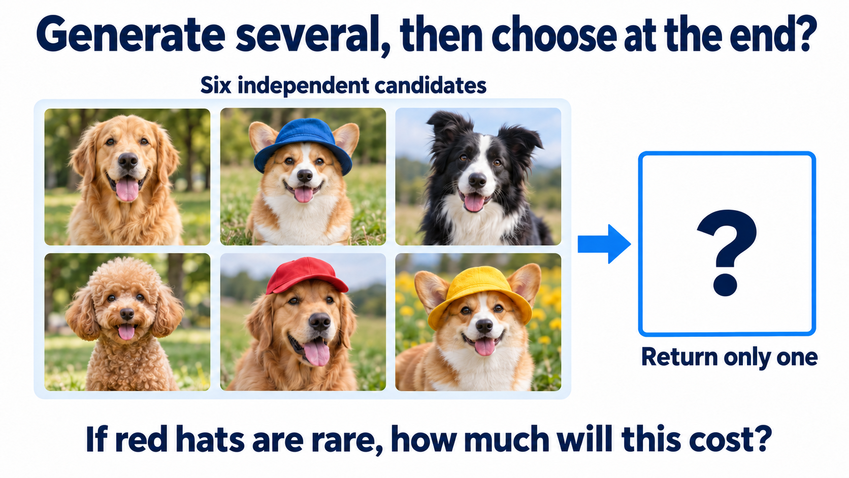
The evaluator only gives scores. How should these drafts continue?
Explore completed-output selection, intermediate SMC, and source MCMC/SPT in your chosen order. Sample, trace ancestry and chains, then build the final comparison.
The user still wants varied dog photos and prefers certain hats, lighting, and compositions. Their scoring program accepts a finished image and returns a number, but cannot say which pixel to change or how. Keep the generative parameters θ fixed. Can scores alone make preferred results appear more often?
Write a finished image as x0 and its reward as R(x0). A scorer that we can query without obtaining usable derivatives is a black-box reward. External simulators, collision checks, and human evaluators can provide such signals. The reward need not be a probability or differentiable.
The score 7 is hypothetical, not a probability or model measurement. Arrows only mean submitting an image and receiving its score. The program provides no direction for revision. What could we do with this number?
Select the image to enlarge
Mugi: draw several, then decide what to keep
MugiA corgi with a Shiba face
“If we do not know how to revise, generate a few images as before. After the evaluator scores them, select one to return. At least we do not need revision directions.”
Mugi keeps each image’s generation unchanged and applies the preference through selection after completion. We could choose the best, or make high scores more likely to be sampled. Do these rules produce the same proportions?
Lumi: keep more copies of promising drafts
LumiA winged deer
“Finishing every image before scoring might be expensive. If we could guess a draft’s future, could we keep more copies of promising drafts and spend less time on the others?”
Lumi wants to change which drafts receive the remaining generation computation. The evaluator still understands only finished images, so intermediate judgments must estimate the future rather than treat noise as a finished photo. Estimates can be wrong; discarding every alternative immediately is risky.
Nori: what if the same draft always yields the same image?
NoriA polar bear in an orca hat
“If the same start always generates the same image, copying a draft only repeats an answer. Could we try different starts and find ones that tend to draw results we like?”
Nori preserves the generation rule and changes which starting points we use. Every new start still requires generation and scoring. Finding a high-scoring start after a few trials does not yet mean sampling a specified distribution.
Which output proportions do we want?
LumiA winged deer
Picking the best is reasonable if we want one high-scoring photo. But the user also wants alternatives. Our question is whether repeated outputs approach this reward tilt:
Here pdata is the base distribution, λ>0 controls reward influence, and ZR averages the reward multiplier over base-generated finished images. Assume 0<ZR<∞; dividing by it restores total mass to 1. Discrete results use probabilities and continuous images use densities. An exact point in the latter need not have a nonzero probability of being sampled.
This target raises high-reward relative weights while retaining base proportions. U7.2 derived its motivation and optimality. Today we ask how to sample, without updating the model. First assume the base sampler exactly produces pdata; we will return to actual model error later.
Data and target shared by all routes
NoriA polar bear in an orca hat
Reuse one executable base: 21N(−2,0.552)+21N(2,0.552). x0 is a completed datum and xt a noisy state. Numbers on the axis are toy data, not live dog photographs. Every route actually samples this distribution and compares it with a numerical reward-tilt reference.
Explore a complete method, then return for the next
Choose the order. Each route includes prediction, actual sampling plots, full derivations, and limitations. Only returning from its final step marks it fully explored. You may return early and resume later.
Select completed outputs: Best-of-N and IW
Keep the highest-scoring image in a batch
MugiA corgi with a Shiba face
“Generate N images and pick the highest score. We can already do that, right?”
Now that Mugi has proposed generating more images, consider this scene. The left side contains separate candidates; only one is returned on the right. Every candidate must be finished and scored.
Select the image to enlarge
Independently generate x0(1),…,x0(N) from the base. Score them, find the highest-scoring index i⋆, and return that image:
i⋆=arg1≤i≤NmaxR(x0(i)),x0=x0(i⋆).
This is Best-of-N. The argmax selects an index; it updates neither pixels nor parameters. Ties can use a fixed or random rule. No reward gradient is needed, and each candidate’s original sampling path is unchanged.
Generate a fresh batch of N, select one, and independently repeat the whole run n times to collect n outputs. N is the candidates compared per run; n is the number of collected outputs. Increasing n reveals this rule’s proportions, which still need to be checked against pR.
Generate candidates and inspect Best-of-N
NoriA polar bear in an orca hat
Actually draw each batch from the mixture and select by reward. Observe rank versus multiplier before calculating the discrete example.
Predict, then inspect the distribution
Increasing N can raise reward. Does that make the output match the dotted reward tilt? What if only λ changes while rankings stay fixed?
A uses N = 1; B uses your N. Each of 1,000 independent batches generates fresh candidates and returns the highest-reward one.
The gray curve shows the original mixture. Running adds actual samples; a reference curve does not establish that it was sampled.
A: settings and observation
B: settings and observation
Fixed baseReference labelled after runningActual samplesA histogram outline
Explain using the plot and numbers
Best-of-N selects by rank. Changing λ without changing ranks leaves winners unchanged, while the tilt changes. More output draws reveal the rule but do not change it into the target. The candidate table records actual draws and selections.
This explains the standard comparison. After changing controls or Python, use the settings and plots you actually ran.
Every candidate is drawn from the same Gaussian mixture. The histogram contains 1,000 independent returns. The dotted curve is a numerical tilt reference, not the theoretical Best-of-N density.
Edit Python and run the experiment yourself
Change the parameters or the sampling rule. Python loads when you press Run and executes in your browser. Each run starts fresh; your edits are not saved.
The first opening imports the controls above; reopening preserves your edits. Settings are imported, not accumulated trained parameters or samples, so finite-sample plots need not match exactly.
The code implements this method and plots its distribution with Matplotlib. The first opening imports current controls; every run samples afresh. Change one parameter at the top. The native plot is not a record of edited Python output.
import math
import numpy as np
import matplotlib.pyplot as plt

# 1. SETTINGS -- change one, run again, and explain the plotted evidence.
strength = 2
N = 8  # candidates per returned sample
reward_kind = "right"  # "right" or "two"
rng = np.random.default_rng(42)
sigma = 0.55
grid = np.linspace(-6, 6, 481)
dx = grid[1] - grid[0]

# 2. FIXED MODEL -- analytic functions, no network training in this cell.
def pdf(x, mu=0.0, var=1.0):
    return np.exp(-0.5 * (x-mu)**2 / var) / np.sqrt(2*np.pi*var)
def R(x):
    return x if reward_kind == "right" else -(np.abs(x)-2.5)**2
def moments(t):
    a = np.exp(-8*t)
    return np.sqrt(a), a*sigma**2 + 1-a
def sample_base(size, t=0.0):
    signal, var = moments(t)
    mu = np.where(rng.random(size) < 0.5, -2.0, 2.0)
    return signal*mu + np.sqrt(var)*rng.normal(size=size)
base = 0.5*pdf(grid, -2, sigma**2)+0.5*pdf(grid, 2, sigma**2)
target = base*np.exp(strength*R(grid))
target /= target.sum()*dx  # finite-grid quadrature reference
reference = target
reference_label = "Tilt reference (quadrature on [-6,6])"
extra_figure = None

# 3. GENERATION -- 1000 independent batches; return ONE sample per batch.
batch = sample_base((1000, N))
rewards = R(batch)
selected = np.argmax(rewards, axis=1)
samples = batch[np.arange(1000), selected]
print("Generated candidates and reward calls:", 1000*N)
print("First batch:", batch[0], "selected index:", selected[0])
print("Finite N does not guarantee the reference tilt.")

# 4. PLOT AND CHECK -- the histogram is from the samples above.
fig, ax = plt.subplots(figsize=(8, 3.6))
ax.plot(grid, base, "--", color="gray", label="Original base")
ax.plot(grid, reference, ":", color="black", label=reference_label)
ax.hist(samples, bins=np.linspace(-6,6,49), weights=np.ones(len(samples))/(len(samples)*0.25), alpha=0.5, label="Actual generated samples")
ax.set(xlabel="clean x0", ylabel="density", xlim=(-6,6))
ax.legend(fontsize=8)
fig.tight_layout()
print("Outputs:", len(samples), "mean:", np.mean(samples), "right share:", np.mean(samples > 0))
print("Outside the plotted window:", np.sum(np.abs(samples)>6))
plt.show()
Package messages and warnings
If either candidate is C, does C win?
MugiA corgi with a Shiba face
Simplify results to A,B,C, each with base probability 1/3. Applying eλR to the scores gives multipliers 1,2,7. These are multipliers, not raw rewards, and C has the highest reward. The desired target probabilities are 1/10,2/10,7/10.
Generate only two candidates each run: Best-of-2. What is the probability of returning C? Compute the probability that neither is C, then take the complement. Does the result equal the target’s 7/10?
You can also think first, then read the explanation. Your writing stays on this page and disappears when you reload.
Calculate the actual output proportions
MugiA corgi with a Shiba face
The candidates are independent, and C wins whenever present. Thus
Returning A requires two copies of A. Returning B requires no C but at least one B. These probabilities sum to 1 but do not have the desired ratio 1:2:7. Best-of-N depends on beating other candidates; reward tilting depends on base weights times multipliers.
Even changing multiplier 7 to 70 leaves Best-of-2 unchanged if the ranking stays the same. The target ratio would become 1:2:70. A ranking-only rule cannot generally preserve multiplier information.
Where do repeated runs lead?
NoriA polar bear in an orca hat
Keep Best-of-2, generate fresh batches every day, and collect one hundred thousand outputs. Which quantity will the frequency of C approach?
Each run still returns C with probability five ninths. More collected outputs do not change that rule.
Seven tenths is the specified target. Repeating a different output distribution does not turn it into that target.
Each run still compares only two candidates, sometimes without C. We increased repetitions, not candidates per run.
Mugi: what if we do not always pick first place?
MugiA corgi with a Shiba face
“If the table happens to contain one A, one B, and one C, could we select them with probabilities 1/10,2/10,7/10? C would remain common while the others still have a chance.”
This samples by weight conditional on a fixed batch. Real base-generated batches need not contain one of each. Where are the base proportions already represented, and which multiplier should each candidate receive?
Candidates already came from the base. What is missing?
LumiA winged deer
Revisit the partners’ proposals
Common base results are already more likely to enter the batch. To represent pR, we need the target’s relative increase over the sampling source. Where the base is positive, simplify
What cancels? What is shared by every candidate? If we will divide by the batch’s total weight, must that shared constant be computed first?
You can also think first, then read the explanation. Your writing stays on this page and disappears when you reload.
Correct candidate contributions toward new proportions
LumiA winged deer
The base cancels, leaving eλR(x0)/ZR. The shared ZR cancels when normalizing, so candidate i only needs positive weight
ω(i)ωˉ(i)=eλR(x0(i)),=∑ℓ=1Nω(ℓ)ω(i).
Here ω(i) is a relative multiplier; ωˉ(i) is the probability of selecting candidate i given this batch. Candidate frequencies already represent the base; selection supplies the reward multiplier. We do not multiply by base probability again.
Correcting contributions by the target-to-source ratio is the core of importance sampling. Here we perform importance weighting (IW), then sample an index with normalized weights and return its finished image.
To estimate a target average, must we select an image?
Let f(x0) be a quantity to average, such as a class indicator, with finite absolute expectation under the target. Multiply and divide the expectation’s integrand by the base density:
Both expectations average base-generated images. The numerator also multiplies by f, and the denominator is ZR. Estimate both means with the same N independent candidates; their factors 1/N cancel:
EpR[f]≈i=1∑Nωˉ(i)f(x0(i)).
This is self-normalized importance sampling. Compute a weighted average directly, without selecting another image. Finite-sample ratios are generally biased. With independent candidates and the relevant integrability, increasing N makes both sample means converge to their expectations, and their ratio to the target average.
Sample candidates by their multipliers
NoriA polar bear in an orca hat
Replace argmax with sampling a normalized-weight index in each fresh batch. Compare N = 1 and larger N and inspect the target approximation.
Predict, then inspect the distribution
Candidates already come from the base. How does selecting by exponential multipliers differ between N = 1 and a larger N?
A uses N = 1; B uses your N. Draw fresh candidates in every batch, normalize their multipliers, and sample one index.
The gray curve shows the original mixture. Running adds actual samples; a reference curve does not establish that it was sampled.
A: settings and observation
B: settings and observation
Fixed baseReference labelled after runningActual samplesA histogram outline
Explain using the plot and numbers
At N = 1 the only normalized weight is 1, so output remains the base. More candidates improve coverage, but finite self-normalized resampling is still approximate. Conditional selection within one batch differs from the output law across batches.
This explains the standard comparison. After changing controls or Python, use the settings and plots you actually ran.
Base frequencies are already represented by candidate generation. Weights supply exp(λR), without multiplying the base density again. Each of 1,000 batches returns one actual sampled candidate.
Edit Python and run the experiment yourself
Change the parameters or the sampling rule. Python loads when you press Run and executes in your browser. Each run starts fresh; your edits are not saved.
The first opening imports the controls above; reopening preserves your edits. Settings are imported, not accumulated trained parameters or samples, so finite-sample plots need not match exactly.
The code implements this method and plots its distribution with Matplotlib. The first opening imports current controls; every run samples afresh. Change one parameter at the top. The native plot is not a record of edited Python output.
import math
import numpy as np
import matplotlib.pyplot as plt

# 1. SETTINGS -- change one, run again, and explain the plotted evidence.
strength = 2
N = 8  # candidates per returned sample
reward_kind = "right"  # "right" or "two"
rng = np.random.default_rng(42)
sigma = 0.55
grid = np.linspace(-6, 6, 481)
dx = grid[1] - grid[0]

# 2. FIXED MODEL -- analytic functions, no network training in this cell.
def pdf(x, mu=0.0, var=1.0):
    return np.exp(-0.5 * (x-mu)**2 / var) / np.sqrt(2*np.pi*var)
def R(x):
    return x if reward_kind == "right" else -(np.abs(x)-2.5)**2
def moments(t):
    a = np.exp(-8*t)
    return np.sqrt(a), a*sigma**2 + 1-a
def sample_base(size, t=0.0):
    signal, var = moments(t)
    mu = np.where(rng.random(size) < 0.5, -2.0, 2.0)
    return signal*mu + np.sqrt(var)*rng.normal(size=size)
base = 0.5*pdf(grid, -2, sigma**2)+0.5*pdf(grid, 2, sigma**2)
target = base*np.exp(strength*R(grid))
target /= target.sum()*dx  # finite-grid quadrature reference
reference = target
reference_label = "Tilt reference (quadrature on [-6,6])"
extra_figure = None

# 3. GENERATION -- 1000 independent batches; return ONE sample per batch.
batch = sample_base((1000, N))
rewards = R(batch)
weights = np.exp(strength*(rewards-rewards.max(axis=1, keepdims=True)))
weights /= weights.sum(axis=1, keepdims=True)
selected = np.sum(rng.random((1000, 1)) > np.cumsum(weights, axis=1), axis=1).clip(0, N-1)
samples = batch[np.arange(1000), selected]
print("Generated candidates and reward calls:", 1000*N)
print("First batch:", batch[0], "selected index:", selected[0])
print("Finite N does not guarantee the reference tilt.")

# 4. PLOT AND CHECK -- the histogram is from the samples above.
fig, ax = plt.subplots(figsize=(8, 3.6))
ax.plot(grid, base, "--", color="gray", label="Original base")
ax.plot(grid, reference, ":", color="black", label=reference_label)
ax.hist(samples, bins=np.linspace(-6,6,49), weights=np.ones(len(samples))/(len(samples)*0.25), alpha=0.5, label="Actual generated samples")
ax.set(xlabel="clean x0", ylabel="density", xlim=(-6,6))
ax.legend(fontsize=8)
fig.tight_layout()
print("Outputs:", len(samples), "mean:", np.mean(samples), "right share:", np.mean(samples > 0))
print("Outside the plotted window:", np.sum(np.abs(samples)>6))
plt.show()
Package messages and warnings
What chance does C have in this batch?
MugiA corgi with a Shiba face
This run produced A,A,C, with multipliers 1,1,7. Given this batch, what is the probability of returning C?
Normalization uses this batch’s total weight. There is no B in this run to add to the denominator.
Weighted sampling can still select A. Only maximization would always select C from this batch.
Target proportions versus this batch
NoriA polar bear in an orca hat
7/10 is the proportion of C in the whole target. Our table contains only A,A,C, with total weight 9, and no weight from B. Selection given this batch can only choose among its members.
The extreme case is N=1: regardless of weight, there is only one candidate, so the output remains the base. Weighted sampling approximates the target with finite candidates; it does not exactly reproduce pR in every batch.
The selection changed. Which costs remain?
NoriA polar bear in an orca hat
Each run now independently generates N base images, scores them, computes multipliers, normalizes, and samples one. More repetitions n reveal the fixed-N output law. More candidates N can improve base coverage and the finite-candidate approximation.
But every candidate must still be completed and scored. If each matches the request with probability p, the chance of at least one hit among N independent candidates is 1−(1−p)N. For p=0.001 and N=1000, it is only about 0.632. This concerns a hit somewhere in the batch, not the probability that the weighted selection succeeds.
Mugi has put scores into selection, but Lumi’s cost question remains: could later computation go to another draft when one already looks unpromising halfway through?
Completed-output selection explored
NoriA polar bear in an orca hat
You implemented Best-of-N and IW and read candidate weights, finite-N output laws, repeated runs, and generation cost. Return to explore intermediate computation or source sampling.
Resample drafts: SMC and the full FK derivation
Lumi: first estimate its eventual score
LumiA winged deer
“Ask the denoiser for a predicted finished image, then show the evaluator. Or complete the same draft independently several times and average the resulting multipliers. Could we compare drafts before finishing?”
We can try, while separating estimates from outcomes. The current noisy state is xt, its denoised estimate is x^0(xt,t), and only reaching the endpoint gives x0. In the VP representation, for αˉt>0,
x^0(xt,t)=αˉtxt−σtϵθ(xt,t).
Here ϵθ is predicted noise and σt=1−αˉt is its amplitude. Subtract predicted noise and divide out the signal scale to get a clean estimate. This is not an already determined future image.
Estimating future weight with eλR(x^0) only queries reward, without differentiation. With multiple independent completions, compute each eλR first, then average. Those trial completions also cost generation. Both are intermediate estimates, not guaranteed exact future averages.
What does the intermediate number tell us?
NoriA polar bear in an orca hat
Revisit the partners’ proposals
Lumi shows a denoised estimate to the evaluator and receives a high score. How can we use that number now?
The scored input is a predicted completion. This avoids gradients but retains uncertainty about the future.
The scored input is an estimate, not the image actually reached at the endpoint. They may differ greatly at high noise.
Returning a score does not imply a derivative with respect to the noisy image. We are comparing candidates.
How should three places be allocated?
LumiA winged deer
Suppose the positive incremental weights for three drafts are 1,2,7, normalizing to 0.1,0.2,0.7. We want three candidates for the next segment, drawing a draft with these probabilities each time, allowing repeated selections.
Across three draws, how many copies does the third draft receive on average? Must every run contain exactly that number? Separate expected copies from actual copies.
You can also think first, then read the explanation. Your writing stays on this page and disappears when you reload.
Draw indices, then continue those drafts
LumiA winged deer
Each draw selects the third draft with probability 0.7, giving expected count 3×0.7=2.1. The first two have expected counts 0.3,0.6, but actual counts are integers. One run might draw (A,C,C) or three copies of C. These are possible outcomes, not prescribed copying lists.
Drawing candidates again by probability is resampling. Afterward, each copy receives equal weight 1/3. Higher-weight drafts have more descendants on average and receive more future computation; the total remains three. Neither model nor scorer is retrained.
For now, 1,2,7 were assumed incremental multipliers for this segment. We still need to derive how future estimates give those incremental weights.
Compare again after each segment
LumiA winged deer
Call an in-progress candidate a particle and keep M simultaneously. Diffusion generates from high noise toward t=0. Choose checkpoints T=tK>⋯>t0=0, where K counts segments and xtk(i) is draft i at time tk.
From tk to tk−1, first move each draft with the original reverse sampler: propagate. Compute its incremental weight ωk−1(i): weight. Normalize over the batch to get ωˉk−1(i), then draw M indices with those probabilities: resample.
Repeating “propagate → weight → resample” is the basic operation of Sequential Monte Carlo (SMC). Here every checkpoint resamples, resetting weights to 1/M. At t=0, uniformly select one of the final M images to return. We change which candidates have descendants, not θ.
Step through which drafts leave descendants
NoriA polar bear in an orca hat
Each particle has a position and ancestor. Step through one population, then draw one return from each of 300 independent populations. Deliberately misestimate H and inspect whether terminal reward correction can restore a lost mode. The full ratio derivation follows.
Predict, then inspect the distribution
If an intermediate estimate wrongly favors only the right, can finite particles retain the left peak after terminal correction? Which share ancestors?
A uses the posterior multiplier; B uses a deliberately right-biased intermediate estimate. M, checkpoints, terminal reward, and seeds stay fixed.
You can inspect one population first. Each click performs one action: propagate → incremental weights → resample.
The gray curve shows the original mixture. Running adds actual samples; a reference curve does not establish that it was sampled.
A: settings and observation
B: settings and observation
Fixed baseReference labelled after runningActual samplesA histogram outline
Explain using the plot and numbers
Each child divides by its own parent’s H; the terminal H uses the actual exp(λR), so intermediate H values telescope on ideal paths. Finite M can still lose a mode, and increasing M need not improve every seed. Colors track one population; the main histogram returns one sample from each of 300 independent populations, not independent descendants within one run.
This explains the standard comparison. After changing controls or Python, use the settings and plots you actually ran.
This toy uses exact reverse conditionals of the known mixture VP process, isolating finite-particle and estimator effects. H_K = 1 and H_0 = exp(λR). Each stage normalizes incremental weights and multinomially resamples M particles. Posterior H uses an analytic integral, without hidden rollouts.
Edit Python and run the experiment yourself
Change the parameters or the sampling rule. Python loads when you press Run and executes in your browser. Each run starts fresh; your edits are not saved.
The first opening imports the controls above; reopening preserves your edits. Settings are imported, not accumulated trained parameters or samples, so finite-sample plots need not match exactly.
The code implements this method and plots its distribution with Matplotlib. The first opening imports current controls; every run samples afresh. Change one parameter at the top. The native plot is not a record of edited Python output.
import math
import numpy as np
import matplotlib.pyplot as plt

# 1. SETTINGS -- change one, run again, and explain the plotted evidence.
strength = 2
M = 24  # particles per population
estimator = "posterior"  # "posterior", "plugin", "misleading"
checkpoints = 6
reward_kind = "two"  # "right" or "two"
rng = np.random.default_rng(42)
sigma = 0.55
grid = np.linspace(-6, 6, 481)
dx = grid[1] - grid[0]

# 2. FIXED MODEL -- analytic functions, no network training in this cell.
def pdf(x, mu=0.0, var=1.0):
    return np.exp(-0.5 * (x-mu)**2 / var) / np.sqrt(2*np.pi*var)
def Phi(x):
    return 0.5 * (1 + np.vectorize(math.erf)(np.asarray(x) / np.sqrt(2)))
def R(x):
    return x if reward_kind == "right" else -(np.abs(x)-2.5)**2
def moments(t):
    a = np.exp(-8*t)
    return np.sqrt(a), a*sigma**2 + 1-a
def sample_base(size, t=0.0):
    signal, var = moments(t)
    mu = np.where(rng.random(size) < 0.5, -2.0, 2.0)
    return signal*mu + np.sqrt(var)*rng.normal(size=size)
def sigmoid(v):
    return np.exp(-np.logaddexp(0, -v))
def post_params(x, t):
    signal, var = moments(t)
    right = sigmoid(4*signal*x/var)
    gain = signal*sigma**2/var
    left_mu = -2 + gain*(x + 2*signal)
    right_mu = 2 + gain*(x - 2*signal)
    variance = sigma**2*(1-np.exp(-8*t))/var
    return right, left_mu, right_mu, variance
def posterior_mean(x, t):
    w, m0, m1, v = post_params(x, t)
    return (1-w)*m0+w*m1
def h(x, t):
    if t == 0:
        return np.exp(strength*R(x))
    w, m0, m1, v = post_params(x, t)
    if reward_kind == "right":
        return (1-w)*np.exp(strength*m0+0.5*strength**2*v)+w*np.exp(strength*m1+0.5*strength**2*v)
    d = 1+2*strength*v
    def component(mu):
        result = 0.0
        for side in [-1, 1]:
            center = (mu+2*strength*v*side*2.5)/d
            factor = np.exp(-strength*(mu-side*2.5)**2/d)/np.sqrt(d)
            result += factor*Phi(side*center/np.sqrt(v/d))
        return result
    return (1-w)*component(m0)+w*component(m1)
base = 0.5*pdf(grid, -2, sigma**2)+0.5*pdf(grid, 2, sigma**2)
target = base*np.exp(strength*R(grid))
target /= target.sum()*dx  # finite-grid quadrature reference
reference = target
reference_label = "Tilt reference (quadrature on [-6,6])"
extra_figure = None

# 3. SMC -- exact reverse transitions of the known mixture; finite M resampling.
def reverse_base(x, current_t, next_t):
    sig0, var0 = moments(next_t)
    sig1, var1 = moments(current_t)
    r = np.exp(-4*(current_t-next_t))
    right = sigmoid(4*sig1*x/var1)
    mu = np.where(rng.random(x.shape) < right, 2.0, -2.0)
    gain = r*var0/var1
    return sig0*mu+gain*(x-sig1*mu)+np.sqrt(max(0, var0-gain*gain*var1))*rng.normal(size=x.shape)
def H(x, t):
    if t == 1:
        return np.ones_like(x)  # H_K = 1
    if t == 0:
        return np.exp(strength*R(x))  # actual terminal reward
    if estimator == "posterior":
        return np.maximum(1e-100, h(x, t))
    if estimator == "plugin":
        return np.maximum(1e-100, np.exp(strength*R(posterior_mean(x, t))))
    return np.exp(np.clip(4*strength*x, -100, 100))  # deliberately wrong intermediate estimate
runs = 300
x = sample_base((runs, M), 1.0)
ancestor = np.tile(np.arange(M), (runs, 1))
trace = [x[0].copy()]
lineage = [ancestor[0].copy()]
for k in range(checkpoints):
    t = 1-k/checkpoints
    next_t = 0 if k+1 == checkpoints else 1-(k+1)/checkpoints
    proposed = reverse_base(x, t, next_t)
    log_weights = np.log(H(proposed, next_t))-np.log(H(x, t))
    weights = np.exp(log_weights-log_weights.max(axis=1, keepdims=True))
    weights /= weights.sum(axis=1, keepdims=True)
    # Each proposed child is divided by its OWN parent's H before resampling.
    cdf = np.cumsum(weights, axis=1)
    parents = np.stack([np.searchsorted(cdf[i], rng.random(M)).clip(0, M-1) for i in range(runs)])
    x = np.take_along_axis(proposed, parents, axis=1)
    ancestor = np.take_along_axis(ancestor, parents, axis=1)
    trace.append(x[0].copy())
    lineage.append(ancestor[0].copy())
# ONE output from each independent population, not 300*M independent descendants.
samples = x[np.arange(runs), rng.integers(M, size=runs)]
print("Independent populations:", runs, "particles each:", M)
print("Reverse transitions:", runs*M*checkpoints, "H calls:", 2*runs*M*checkpoints)
print("Surviving ancestors in the first population:", len(np.unique(ancestor[0])))
extra_figure, ax = plt.subplots(figsize=(8, 3.2))
for i, (positions, origins) in enumerate(zip(trace, lineage)):
    ax.scatter(positions, np.full(M, i), c=origins, cmap="tab20", s=15, vmin=0, vmax=max(1,M-1))
ax.set(xlabel="noisy state x_t (last row is clean)", ylabel="checkpoint in generation order")
ax.invert_yaxis()
extra_figure.tight_layout()

# 4. PLOT AND CHECK -- the histogram is from the samples above.
fig, ax = plt.subplots(figsize=(8, 3.6))
ax.plot(grid, base, "--", color="gray", label="Original base")
ax.plot(grid, reference, ":", color="black", label=reference_label)
ax.hist(samples, bins=np.linspace(-6,6,49), weights=np.ones(len(samples))/(len(samples)*0.25), alpha=0.5, label="Actual generated samples")
ax.set(xlabel="clean x0", ylabel="density", xlim=(-6,6))
ax.legend(fontsize=8)
fig.tight_layout()
print("Outputs:", len(samples), "mean:", np.mean(samples), "right share:", np.mean(samples > 0))
print("Outside the plotted window:", np.sum(np.abs(samples)>6))
plt.show()
Package messages and warnings
What does copying only the best overlook?
MugiA corgi with a Shiba face
Mugi says, “To spend time on good drafts, why not keep only the highest-scoring one and copy it M times?” What does this overlook?
Finite candidates need exploration. We score an estimated future, not a known best final path.
Parameters remain fixed. Keeping one ancestor changes candidates and computation allocation, not model training.
Which rule follows the copied draft?
NoriA polar bear in an orca hat
With fresh sampler randomness, copies of one draft may reach different results. Along the same deterministic ODE, however, identical states follow the same route. Ten copies still give one answer.
Shrinking to a few ancestors and narrowing exploration is particle degeneracy. Random normalized-weight resampling can also cause it, especially with concentrated weights. Any added exploration or perturbation must be checked for target preservation; copy count alone does not establish diversity.
Would multiplying future scores every time overcount?
NoriA polar bear in an orca hat
Having only a few ancestors and narrowing exploration is particle degeneracy. Random resampling can still cause it when weights concentrate. Copies need later randomness to separate; under the same deterministic rule, more copies do not create different answers.
“We know how to resample. But suppose a draft’s future multiplier is first estimated as 2, then is 6 at completion. Multiplying by both 2 and 6 gives 12, although we only wanted a factor of 6. What was counted twice?”
Let Hk(xtk) be a positive estimate at checkpoint tk. It may be a cheap estimate, not U7.2’s exact posterior average. Set HK≡1 at the start and H0(x0)=eλR(x0) at completion, with positive intermediate values.
Each complete base path should receive the terminal multiplier only once. We are checking the accumulated product, not how high each separate estimate is. First follow a worked example, then choose the next operation yourself.
Watch how we choose the next mathematical operation
NoriA polar bear in an orca hat
Split this path into two segments: H2=1, H1=2, and H0=6. Open one operation at a time and see how the goal determines the tool.
From cumulative multipliers to each segment’s increase
Bring the cumulative multiplier to the intermediate estimate
Goal
At the first checkpoint, the cumulative multiplier should be 2.
Tool
Divide the new estimate by the multiplier already accumulated.
Why this tool
We start at 1 and need the missing factor that brings it to 2.
Solve “1 times what equals 2?” The first multiplier is
H2H1=12=2.
Here H1,H2 are the same path’s estimates at its two checkpoints. It has already accumulated a factor of 2; the next segment cannot pretend otherwise.
Supply only the factor still missing in the second segment
Goal
We already have a factor of 2 and want a final factor of 6.
Tool
Solve the multiplication relation by dividing 6 by 2.
Why this tool
We need a multiplicative factor, not an additive increase in score.
Solve “2 times what equals 6?” The increment is
H1H0=26=3.
Multiplying directly by 6 would give 12; the difference 4 is not the missing factor either. We divide because the unknown is a factor in a product.
Multiply both segments and check for double counting
Goal
The entire path should receive only the final factor of 6.
Tool
Multiply and cancel the shared intermediate estimate.
Why this tool
The intermediate 2 appears in one numerator and the next denominator.
Connect the segments:
H2H1H1H0=1226=6.
The intermediate estimate helps allocate computation, then cancels against the next ratio. Reward is not ignored; the same terminal preference accumulates only once.
Choose the next mathematical tool
NoriA polar bear in an orca hat
Try another path: its previous checkpoint has accumulated a factor of 3, and the new estimate calls for 12. Which multiplier should this segment add? First identify the missing multiplicative factor, then choose a tool.
The new-to-old ratio supplies only what the cumulative product lacks, without recounting the previous part.
The difference 9 is additive. Multiplying the existing 3 by it gives 27 rather than the desired 12.
An existing factor of 3 times 12 accumulates to 36, counting the earlier contribution again.
Given the framework, can you fill in the cancellation?
NoriA polar bear in an orca hat
Now split one path into three segments. Its positive estimates from start through two intermediate checkpoints to finish are H3,H2,H1,H0. For now these denote values along that one path; we will restore state inputs shortly.
Each segment uses new divided by old, giving the product
H3H2H2H1H1H0.
Which terms cancel, and what remains? With start value 1 and the true terminal reward multiplier, explain why intermediate estimates need not be exact to preserve the ideal full-path multiplier.
You can also think first, then read the explanation. Your writing stays on this page and disappears when you reload.
Each segment adds only the new ratio
NoriA polar bear in an orca hat
In the three-segment product, H2,H1 each appear once above and below the fraction bar, leaving H0/H3. Restore the segment states and check the needed conditions.
From ratios along one path to the terminal multiplier
Compare consecutive states on the same path
Goal
Define the multiplier for the segment from t_k to t_{k−1}.
Tool
Take the ratio of the new estimate to the old one.
Why this tool
The new candidate must be paired with its actual predecessor to correct the same path’s cumulative weight.
Call this segment’s multiplier function a potential:
Gk−1(xtk−1,xtk)=Hk(xtk)Hk−1(xtk−1).
The numerator is the estimate after the segment, and the denominator is the estimate before it. Dividing by another draft’s old estimate would destroy the matching values needed for cancellation.
Substitute candidate i’s states
Goal
Compute this draft’s sampling weight for the segment.
Tool
Evaluate the potential at the candidate’s consecutive states.
Why this tool
The potential describes the rule; resampling needs a numerical value for each candidate.
Our main construction uses the original sampler for this segment, so candidate i has incremental weight
ωk−1(i)=Gk−1(xtk−1(i),xtk(i)).
Normalize by the sum of this batch’s ω values to obtain selection probabilities. A different proposal also requires correcting the sampling source; an extra section below expands that ratio.
Multiply along one ancestral path
Goal
Check the multiplier accumulated over every segment.
Tool
Cancel matching factors in the product.
Why this tool
Each intermediate H appears in adjacent segments’ numerator and denominator.
Multiply segment ratios along the same ancestral path. As in the three-segment example, intermediate values cancel, leaving
k=1∏KGk−1(xtk−1,xtk)=HK(xT)H0(x0).
This checks a product along one path, not an average across particles. Different paths have their own intermediate states and estimates.
Insert the start and endpoint conditions
Goal
Leave only the finished image’s true reward multiplier.
Tool
Substitute H_K=1 and the terminal exponential weight.
Why this tool
Cancellation gives H_0/H_K; matching the desired multiplier depends on how those endpoints are chosen.
Set HK≡1 and H0(x0)=eλR(x0). Then
HK(xT)H0(x0)=eλR(x0).
Intermediate estimates allocate computation; endpoint choices determine the accumulated multiplier. Positive estimates make the ratios defined. This construction preserves the ideal terminal tilt, but finite-M drafts may have been discarded already, so actual approximation still depends on those estimates.
How do path multipliers give finished-image proportions?
LumiA winged deer
Each path now receives only eλR(x0). Yet multiple paths may reach the same finished result. What mathematical operation gives that result’s probability in the new distribution?
Every compatible path can contribute, retaining its original path probability.
Keeping only the most likely path removes contributions from other paths to the same endpoint. That selects a path rather than calculating total probability.
Base paths need not be equally likely. Equally averaging multipliers while discarding path probabilities loses the base proportions.
First add the contributions of four paths
NoriA polar bear in an orca hat
Try a four-path base example: two paths reach A with probabilities 0.1,0.2; two reach B with probabilities 0.3,0.4. Terminal multipliers are 1 for A and 3 for B. The weighted masses are
A:B:0.1⋅1+0.2⋅1=0.3,0.3⋅3+0.4⋅3=2.1.
A shared terminal multiplier can leave the sum. Equivalently, first add base path probabilities to obtain pdata(A)=0.3 and pdata(B)=0.7, then multiply by 1,3. The normalizing total is 2.4, giving probabilities 1/8,7/8.
This is why we chose “accumulate all paths.” Keeping one path would omit the other’s mass.
Specify path proportions before actually sampling
LumiA winged deer
Use the original sampler’s path distribution P to connect full-path multipliers with finished-image proportions. Write the checkpoint sequence as xtK:0. First define a path target PR, then check its endpoint distribution.
Weight paths, then accumulate intermediate possibilities
Reweight each base path
Goal
Define the desired relative weight of a generation path.
Tool
Multiply original path mass by segment potentials and normalize.
Why this tool
Multipliers alone are not probabilities. Preserve original contributions and restore total mass to 1.
PR(dxtK:0)=ZR1P(dxtK:0)k=1∏KGk−1.
Here P(dxtK:0) denotes the base probability measure on these paths. The product uses the state inputs defined above. The total weighted base-path mass ZR is assumed finite and nonzero.
Insert the accumulated multiplier we already checked
Goal
Identify which reward a complete path ultimately depends on.
Tool
Replace the potential product with its telescoped result.
Why this tool
Intermediate H values already canceled along this path. They should not be multiplied in again.
PR(dxtK:0)=ZReλR(x0)P(dxtK:0).
The new multiplier depends only on endpoint x0. Any two paths reaching the same result receive the same terminal weight, while retaining their original relative probabilities.
Include every path to the same result
Goal
Calculate terminal proportions from the path distribution.
Tool
Sum over intermediate states, or integrate in continuous spaces.
Why this tool
An endpoint does not tell us which path was taken. All compatible contributions must be included.
The four paths gave weighted masses 0.3 for A and 2.1 for B. At a fixed endpoint every compatible path receives the same terminal multiplier, so factor it out of the sum over intermediate states. Continuous spaces use an integral while retaining each base path’s contribution.
Read back the general terminal target
Goal
Verify that endpoint proportions equal the specified reward tilt.
Tool
Factor out the endpoint-only multiplier and retain the base terminal law.
Why this tool
At a fixed endpoint, the multiplier does not vary with intermediate states. Accumulating them leaves the original sampler’s terminal distribution.
If the base sampler ends at pdata, accumulating all paths for each endpoint, just as in the four-path example, gives
pR(x0)=ZReλR(x0)pdata(x0).
This denotes probabilities for discrete results and densities for continuous ones. We defined path weighting, then derived its terminal target. No particle count M appears in the definition, and no image has yet been sampled.
This potential-weighted path framework is a Feynman–Kac (FK) model. SMC is the finite-particle sampling algorithm approximating it. The derivation specifies an ideal target; finite-draft error and degeneracy require separate checks.
How do FK steering and DAS relate to these two layers?
Singhal and colleagues’ FK steering applies this construction to diffusion guidance: choose intermediate estimates, potentials, proposals, and resampling times, then sample with particle methods. Kim, Kim, and Park’s DAS (Diffusion Alignment as Sampling) also uses SMC, gradually increasing intermediate-target preference through reward tempering.
Relate these names to two layers: how targets and potentials are constructed, and how they are sampled. FK and SMC are not mutually exclusive methods.
With a different proposal, does weight still equal potential?
Our main construction propagates with the original sampler, so proposal and base transition coincide. If another transition density τk−1 proposes states while the base density is pbase, the weight must also correct their ratio. With resampling each segment and equal previous weights,
The first factor is the target’s increase over the base path. The second compensates for drawing from the proposal rather than the base transition, for the same reason as finished-image IW. The proposal must cover regions with target mass for this ratio to work.
Only when τk−1=pbase does the ratio become 1, recovering ω=G. Here Gk−1 is an incremental weight function; below, G(z) is a deterministic generator. Their inputs and subscripts distinguish the roles.
Which layer suffers from a poor intermediate estimate?
LumiA winged deer
An intermediate Hk is poor but remains positive. We keep same-path ratios, HK=1, and the true terminal reward for H0. Which claim follows from the construction?
Accumulated multipliers determine the path target; actual sampling produces finite-particle error and degeneracy.
Poor estimates can eliminate drafts that would later be good. A correct product does not establish sufficient finite-M exploration.
Is the remaining factor really the intended one?
NoriA polar bear in an orca hat
Cancellation leaves H0/HK. If the last reward still scores a predicted image instead of true eλR(x0), the remaining terminal weight may be different.
Likewise, a nonconstant HK(xT) without a matching initial correction leaves an extra 1/HK(xT). More particles can improve approximation, but cannot automatically repair a changed FK target.
Bring the finite drafts to completion
LumiA winged deer
Lumi’s complete procedure is now clear. Draw M original-sampler starts. At each segment, retain old states, propagate, and divide each new H by its own predecessor’s old H. Normalize and independently resample M indices with replacement. Equal-weight copies enter the next segment. At completion, H0 uses the finished image’s true reward.
The final M images define an empirical distribution:
pR(M)(dx0)=M1i=1∑Mδx0(i)(dx0).
Here δx0(i) puts a point mass at image i. Estimate a category’s frequency by counting its members and dividing by M. Equal weights do not imply independent samples, since particles may share ancestors. Uniformly selecting one returns this run’s output.
How do more particles M differ from more fixed-M runs n?
Let f(x0) be a bounded image statistic, such as the indicator of C. With fixed checkpoints, correct weights, and the corresponding integrability conditions, SMC consistency states
The left side averages M particles in one run; the right side is the target average. “In probability” means the probability of exceeding any fixed positive error tolerance tends to 0. It does not require independent particles within the run.
Increasing M improves each run’s FK-target approximation. Independently repeating a fixed-M sampler n times only clarifies its output proportions, which may remain biased. This limit also does not repair an incorrectly specified terminal weight.
Must every segment resample?
No. Effective sample size (ESS) describes concentration of normalized weights:
ESS=∑i=1M(ωˉ(i))21.
With equal weights, the squared sum is M/M2=1/M, giving ESS M. If one weight approaches 1, the squared sum approaches 1, giving ESS near 1. This measures weight concentration, not independent ancestor count.
We can resample only when ESS falls below a threshold. If a segment skips resampling, retain the old weights and multiply by the next incremental potential. Skipping resampling cannot be combined with assuming equal weights at the next segment.
Three particles per run, but ten thousand runs?
NoriA polar bear in an orca hat
Every run uses only M=3 particles, but we repeat independently many times. Is increasing only n enough to eliminate finite-M sampling bias?
The operations and full derivation are complete
NoriA polar bear in an orca hat
You observed resampling and ancestry and read incremental ratios, telescoping potentials, the FK endpoint law, and finite-M error and degeneracy. Check ideal target construction separately from finite sampling performance.
Change the source: MCMC and SPT
The same start always draws the same image
NoriA polar bear in an orca hat
“Back to my proposal: if copied drafts always produce the same image, could we preserve the generation rule and try new starts?”
Write the deterministic generator as G: start z produces x0=G(z). It includes the fixed generation computation; the same z yields the same result. Originally the source has density pZ, so we draw z∼pZ.
Every start has a queryable score R(G(z)). To favor high-scoring outputs, put the multiplier on the source:
pZR(z)∝pZ(z)eλR(G(z)).
The factor pZ retains original relative source densities, while the exponential raises weights for starts yielding high scores. The generation rule stays fixed; the desired source distribution changes. Writing this target does not yet supply a sampler.
What if different starts draw the same result?
NoriA polar bear in an orca hat
Use three discrete starts za,zb,zc, each originally of probability 1/3, with G(za)=A and G(zb)=G(zc)=B. The output multipliers are 1 for A and 3 for B.
The source weights become 1/3,1,1. After normalization, what are the probabilities of generating A,B? Add the probabilities of starts producing the same result, then compare with image-space base times reward.
You can also think first, then read the explanation. Your writing stays on this page and disappears when you reload.
Add all starts that draw the same result
NoriA polar bear in an orca hat
Total source weight is 7/3, giving source probabilities 1/7,3/7,3/7. Only one start produces A, so its probability is 1/7. Two produce B, totaling 6/7.
The original output probabilities were 1/3,2/3. Multiplying by 1,3 gives weights 1/3,2, again normalizing to 1/7,6/7. G need not be one-to-one; include every source producing the same result.
More generally, also write the source normalizer as ZR=Ez∼pZ[eλR(G(z))], the mean reward multiplier of base-generated outputs. Sampling from pZR and applying the same G gives any integrable image statistic f the average
The original z∼pZ followed by G produces the base output law. This equation is exactly its reward-weighted average. Source tilting therefore reweights the generator’s actual output law, without needing image-space density or eliminating original model error.
Try a new start, then decide whether it stays
NoriA polar bear in an orca hat
“We have a source target. Could we propose z′ from the current z, generate G(z′), score it, and decide whether to move there?”
Yes, but always accepting only higher scores again finds high-scoring points rather than specified proportions. A sequence of current and subsequent starts is a chain. Acceptance moves to z′; rejection stays at z. Staying still is also a step.
Using target-preserving Markov transitions to collect samples is Markov chain Monte Carlo (MCMC). First consider a symmetric proposal, equally likely in either direction. The acceptance probability is
Here λj is chain j’s reward strength. Normalizing constants cancel. The ratio compares prior density times reward multiplier. Draw U∼Uniform(0,1); move to z′ if U<Paccept, otherwise keep z. No reward gradient is needed.
Why does this acceptance probability preserve the target?
Denote the chain target by π(z)=pZλj(z) and proposal density by a(z′∣z). Symmetry means a(z′∣z)=a(z∣z′). Forward probability flow is
Exchanging z,z′ gives the same reverse flow by symmetry. Including rejection probability at the current state prevents net target mass from flowing to one side. This equal-flow condition is detailed balance, giving target invariance.
An asymmetric proposal needs the additional ratio a(z∣z′)/a(z′∣z). The prior-and-reward-only version no longer suffices. Target preservation is a transition property; sufficient finite-run exploration is a separate question.
Run a source chain and retain rejected moves
NoriA polar bear in an orca hat
A fixed quantile generator maps standard-Normal sources to the same mixture base. Change only source acceptance and inspect lower-reward accepts, repeated positions, and the actual output histogram.
Predict, then inspect the distribution
Would always accepting only higher reward sample the target? Can the actual acceptance rule accept lower reward?
A uses λ = 0; B uses your λ. Both single chains start at z = -0.8 with identical iteration counts, proposal size, and seed.
The gray curve shows the original mixture. Running adds actual samples; a reference curve does not establish that it was sampled.
A: settings and observation
B: settings and observation
Fixed baseReference labelled after runningActual samplesA histogram outline
Explain using the plot and numbers
Acceptance uses both the standard-Normal prior and reward ratio and can accept lower reward. Repeated states after rejection must be retained; keeping only accepted moves changes the distribution. A finite chain can remain in one mode; 400 warm-up iterations do not certify convergence.
This explains the standard comparison. After changing controls or Python, use the settings and plots you actually ran.
Fixed G(z) = F_base^-1(Phi(z)): Phi is the standard-Normal CDF and F_base is the mixture CDF. Find z’s cumulative probability, then the location with the same cumulative probability in the base. This maps a Normal source to the mixture, always giving the same output for the same z. Numerical inversion does not train a model or differentiate reward. Acceptance uses prior × reward, and the histogram retains rejected and correlated states.
Edit Python and run the experiment yourself
Change the parameters or the sampling rule. Python loads when you press Run and executes in your browser. Each run starts fresh; your edits are not saved.
The first opening imports the controls above; reopening preserves your edits. Settings are imported, not accumulated trained parameters or samples, so finite-sample plots need not match exactly.
The code implements this method and plots its distribution with Matplotlib. The first opening imports current controls; every run samples afresh. Change one parameter at the top. The native plot is not a record of edited Python output.
import math
import numpy as np
import matplotlib.pyplot as plt

# 1. SETTINGS -- change one, run again, and explain the plotted evidence.
strength = 2
steps = 1600
reward_kind = "two"  # "right" or "two"
proposal_step = 0.35
rng = np.random.default_rng(42)
sigma = 0.55
grid = np.linspace(-6, 6, 481)
dx = grid[1] - grid[0]

# 2. FIXED MODEL -- analytic functions, no network training in this cell.
def pdf(x, mu=0.0, var=1.0):
    return np.exp(-0.5 * (x-mu)**2 / var) / np.sqrt(2*np.pi*var)
def R(x):
    return x if reward_kind == "right" else -(np.abs(x)-2.5)**2
base = 0.5*pdf(grid, -2, sigma**2)+0.5*pdf(grid, 2, sigma**2)
target = base*np.exp(strength*R(grid))
target /= target.sum()*dx  # finite-grid quadrature reference
reference = target
reference_label = "Tilt reference (quadrature on [-6,6])"
extra_figure = None

# 3. SOURCE SEARCH -- a fixed quantile generator G; standard-Normal source prior.
def G(z):
    p = min(1-1e-12, max(1e-12, 0.5*(1+math.erf(z/math.sqrt(2)))))
    lo, hi = -8.0, 8.0
    for _ in range(40):
        mid = (lo+hi)/2
        cdf = 0.25*(2+math.erf((mid+2)/(sigma*math.sqrt(2)))+math.erf((mid-2)/(sigma*math.sqrt(2))))
        if cdf < p:
            lo = mid
        else:
            hi = mid
    return (lo+hi)/2
lambdas = [strength]
proposal_steps = [proposal_step]  # step size is a separate choice
states = []
for _ in lambdas:
    x = G(-0.8)
    states.append([-0.8, x, float(R(x))])
samples, trace = [], []
accepted = swaps = lower_accepted = 0
burn = 400
for k in range(steps+burn):
    for j, lam in enumerate(lambdas):
        z, x, old_reward = states[j]
        proposed_z = z+proposal_steps[j]*rng.normal()
        proposed_x = G(proposed_z)
        proposed_reward = float(R(proposed_x))
        log_ratio = -0.5*(proposed_z**2-z**2)+lam*(proposed_reward-old_reward)
        if math.log(max(1e-300, rng.random())) < min(0, log_ratio):
            accepted += 1
            lower_accepted += proposed_reward < old_reward
            states[j] = [proposed_z, proposed_x, proposed_reward]
    if len(states) > 1:
        j = k % 2
        log_ratio = (lambdas[j]-lambdas[j+1])*(states[j+1][2]-states[j][2])
        if math.log(max(1e-300, rng.random())) < min(0, log_ratio):
            states[j], states[j+1] = states[j+1], states[j]  # swap z, G(z), reward together
            swaps += 1
    if k >= burn:
        samples.append(states[-1][1])  # keep rejected/repeated states too
        trace.append([state[0] for state in states])
samples = np.asarray(samples)
print("G and reward evaluations:", len(lambdas)*(steps+burn+1))
print("Accepted:", accepted, "accepted lower rewards:", lower_accepted, "swaps:", swaps)
print("Histogram includes rejections; states are correlated. Burn-in does not certify convergence.")
extra_figure, ax = plt.subplots(figsize=(8, 3.2))
for j, lam in enumerate(lambdas):
    ax.plot(np.asarray(trace)[:,j], label=f"source chain, lambda={lam:g}", alpha=0.8)
ax.set(xlabel="retained iteration (rejections included)", ylabel="source z")
ax.legend(fontsize=8)
extra_figure.tight_layout()

# 4. PLOT AND CHECK -- the histogram is from the samples above.
fig, ax = plt.subplots(figsize=(8, 3.6))
ax.plot(grid, base, "--", color="gray", label="Original base")
ax.plot(grid, reference, ":", color="black", label=reference_label)
ax.hist(samples, bins=np.linspace(-6,6,49), weights=np.ones(len(samples))/(len(samples)*0.25), alpha=0.5, label="Actual generated samples")
ax.set(xlabel="clean x0", ylabel="density", xlim=(-6,6))
ax.legend(fontsize=8)
fig.tight_layout()
print("Outputs:", len(samples), "mean:", np.mean(samples), "right share:", np.mean(samples > 0))
print("Outside the plotted window:", np.sum(np.abs(samples)>6))
plt.show()
Package messages and warnings
Could a slightly lower score still be accepted?
MugiA corgi with a Shiba face
The proposal is symmetric, old and new starts have equal prior density, and the new reward weight is half the old one. How should we decide?
Allowing lower-scoring candidates preserves the forward and reverse probability flows.
Always rejecting lower scores changes the rule into score climbing and loses the target-preservation argument.
The proposal is symmetric, not the target. Reward weights still affect acceptance.
Could another chain help escape one composition?
LumiA winged deer
“If high-scoring starts lie in distant regions, one chain may keep finding the same composition. Could several reward strengths search together and exchange what they find?”
Let chain j use strength λj, targeting
pZλj(z)∝pZ(z)eλjR(G(z)).
A smaller λj is less influenced by reward and can be paired with larger proposal steps to explore other base-supported regions. A larger λj favors high scores and can be paired with smaller steps for refinement. Strength does not automatically determine proposal step size; they are separate design choices.
Each chain first tries local proposals with the acceptance rule, then proposes cross-chain swaps to bring exploratory results to the desired strength. This is Wang and colleagues’ Source Parallel Tempering (SPT): sample several source-space targets at different strengths, with swaps also subject to acceptance. Collect z from the chain at desired strength λ, then output G(z).
Which factors cancel before and after a swap?
LumiA winged deer
Two chains have strengths λi,λj and starts zi,zj. Their joint target is the product of their targets. Swapping the starts gives this reward-dependent new-to-old ratio:
Both sides contain the same pZ(zi)pZ(zj), so prior factors cancel. Combine the exponential’s exponents. Which differences in strengths and rewards multiply together?
You can also think first, then read the explanation. Your writing stays on this page and disappears when you reload.
Swaps must preserve each chain’s proportions too
LumiA winged deer
Subtract denominator exponents from numerator exponents, then factor common terms:
With symmetric selection of swap pairs, this rule preserves the product of chain targets. We cannot simply import another chain’s higher score: that may change the target as well as exploration speed.
One SPT round proposes local starts, generates and scores, accepts or stays using Paccept, then decides a pair’s swap using Pswap. Swap the start and its already computed reward together; do not pair a start with another image’s score.
Every fresh proposal costs generation and scoring. Samples in the desired chain may remain correlated, and we must check coverage of distinct high-reward regions. A target-preserving rule does not establish that finite search has reached the target.
Run three strengths and probabilistic swaps
NoriA polar bear in an orca hat
Compare complete single-chain and three-chain records. Equal iterations per chain cost more G and reward calls with three chains. Inspect traces and coverage of both modes instead of treating higher mean reward as convergence.
Predict, then inspect the distribution
Can swaps between chains of different strengths reach another high-reward region? What extra generation and reward cost do they incur?
A is one chain at the target strength; B uses strengths 0, λ/2, λ with adjacent swaps. Iterations per chain match, so B has three times the evaluation cost; this is not an equal-budget comparison.
The gray curve shows the original mixture. Running adds actual samples; a reference curve does not establish that it was sampled.
A: settings and observation
B: settings and observation
Fixed baseReference labelled after runningActual samplesA histogram outline
Explain using the plot and numbers
Each chain makes an MCMC proposal, then swaps z, output, and reward together according to the swap ratio. Collect only the λ chain; do not mix in low-strength samples. Larger proposals are separately configured, not generated by λ. Finite runs can still explore poorly.
This explains the standard comparison. After changing controls or Python, use the settings and plots you actually ran.
The same fixed quantile generator. Proposal standard deviations are 1.4, 0.8, and your target-chain step size. Swap probability is min(1, exp[(λ_i−λ_j)(R_j−R_i)]). The trace shows source z across iterations, not diffusion time.
Edit Python and run the experiment yourself
Change the parameters or the sampling rule. Python loads when you press Run and executes in your browser. Each run starts fresh; your edits are not saved.
The first opening imports the controls above; reopening preserves your edits. Settings are imported, not accumulated trained parameters or samples, so finite-sample plots need not match exactly.
The code implements this method and plots its distribution with Matplotlib. The first opening imports current controls; every run samples afresh. Change one parameter at the top. The native plot is not a record of edited Python output.
import math
import numpy as np
import matplotlib.pyplot as plt

# 1. SETTINGS -- change one, run again, and explain the plotted evidence.
strength = 2
steps = 1600
reward_kind = "two"  # "right" or "two"
proposal_step = 0.35
rng = np.random.default_rng(42)
sigma = 0.55
grid = np.linspace(-6, 6, 481)
dx = grid[1] - grid[0]

# 2. FIXED MODEL -- analytic functions, no network training in this cell.
def pdf(x, mu=0.0, var=1.0):
    return np.exp(-0.5 * (x-mu)**2 / var) / np.sqrt(2*np.pi*var)
def R(x):
    return x if reward_kind == "right" else -(np.abs(x)-2.5)**2
base = 0.5*pdf(grid, -2, sigma**2)+0.5*pdf(grid, 2, sigma**2)
target = base*np.exp(strength*R(grid))
target /= target.sum()*dx  # finite-grid quadrature reference
reference = target
reference_label = "Tilt reference (quadrature on [-6,6])"
extra_figure = None

# 3. SOURCE SEARCH -- a fixed quantile generator G; standard-Normal source prior.
def G(z):
    p = min(1-1e-12, max(1e-12, 0.5*(1+math.erf(z/math.sqrt(2)))))
    lo, hi = -8.0, 8.0
    for _ in range(40):
        mid = (lo+hi)/2
        cdf = 0.25*(2+math.erf((mid+2)/(sigma*math.sqrt(2)))+math.erf((mid-2)/(sigma*math.sqrt(2))))
        if cdf < p:
            lo = mid
        else:
            hi = mid
    return (lo+hi)/2
lambdas = [0.0, strength/2, strength]
proposal_steps = [1.4, 0.8, proposal_step]  # step size is a separate choice
states = []
for _ in lambdas:
    x = G(-0.8)
    states.append([-0.8, x, float(R(x))])
samples, trace = [], []
accepted = swaps = lower_accepted = 0
burn = 400
for k in range(steps+burn):
    for j, lam in enumerate(lambdas):
        z, x, old_reward = states[j]
        proposed_z = z+proposal_steps[j]*rng.normal()
        proposed_x = G(proposed_z)
        proposed_reward = float(R(proposed_x))
        log_ratio = -0.5*(proposed_z**2-z**2)+lam*(proposed_reward-old_reward)
        if math.log(max(1e-300, rng.random())) < min(0, log_ratio):
            accepted += 1
            lower_accepted += proposed_reward < old_reward
            states[j] = [proposed_z, proposed_x, proposed_reward]
    if len(states) > 1:
        j = k % 2
        log_ratio = (lambdas[j]-lambdas[j+1])*(states[j+1][2]-states[j][2])
        if math.log(max(1e-300, rng.random())) < min(0, log_ratio):
            states[j], states[j+1] = states[j+1], states[j]  # swap z, G(z), reward together
            swaps += 1
    if k >= burn:
        samples.append(states[-1][1])  # keep rejected/repeated states too
        trace.append([state[0] for state in states])
samples = np.asarray(samples)
print("G and reward evaluations:", len(lambdas)*(steps+burn+1))
print("Accepted:", accepted, "accepted lower rewards:", lower_accepted, "swaps:", swaps)
print("Histogram includes rejections; states are correlated. Burn-in does not certify convergence.")
extra_figure, ax = plt.subplots(figsize=(8, 3.2))
for j, lam in enumerate(lambdas):
    ax.plot(np.asarray(trace)[:,j], label=f"source chain, lambda={lam:g}", alpha=0.8)
ax.set(xlabel="retained iteration (rejections included)", ylabel="source z")
ax.legend(fontsize=8)
extra_figure.tight_layout()

# 4. PLOT AND CHECK -- the histogram is from the samples above.
fig, ax = plt.subplots(figsize=(8, 3.6))
ax.plot(grid, base, "--", color="gray", label="Original base")
ax.plot(grid, reference, ":", color="black", label=reference_label)
ax.hist(samples, bins=np.linspace(-6,6,49), weights=np.ones(len(samples))/(len(samples)*0.25), alpha=0.5, label="Actual generated samples")
ax.set(xlabel="clean x0", ylabel="density", xlim=(-6,6))
ax.legend(fontsize=8)
fig.tight_layout()
print("Outputs:", len(samples), "mean:", np.mean(samples), "right share:", np.mean(samples > 0))
print("Outside the plotted window:", np.sum(np.abs(samples)>6))
plt.show()
Package messages and warnings
Does each new start require learning again?
NoriA polar bear in an orca hat
SPT generates and scores again for each new proposed start. Can all these operations preserve the generative parameters θ?
Source targets, acceptance, and swaps explored
NoriA polar bear in an orca hat
You implemented MCMC and SPT and read how source tilting yields output laws, acceptance and swap derivations, finite-search limits, and generation cost. Return before comparing all methods under different constraints.
Back at the workbench: what does each approach change?
NoriA polar bear in an orca hat
The method names are now familiar. Place each action and limitation where it belongs. Read each row’s explanation before continuing.
Final selection · Scoring Score a batch of finished images, then decide which to return.
Intermediate SMC · Scoring Estimate future multipliers from drafts to decide which descendants continue.
Source SPT · Scoring Generate from a proposed start, score, then decide whether to change starts.
Final selection · Rule Pick the highest score, or normalize exponential weights and sample one.
Intermediate SMC · Rule Resample M copies with corrected incremental weights, allowing shared ancestors.
Source SPT · Rule Accept starts using target ratios and swap using acceptance probabilities.
Final selection · Computation Rare targets need many candidates; finite-N IW still has approximation error.
Intermediate SMC · Computation Check estimates and ancestor concentration; larger M cannot fix a wrong target.
Source SPT · Computation Every proposal needs completion and scoring; finite search may stay local.
What if generation can pause at checkpoints?
NoriA polar bear in an orca hat
You can save noisy states, advance each by a segment, and cheaply estimate future multipliers. Which operation directly reallocates computation before completion?
These are SMC’s interface prerequisites; estimator quality and degeneracy still require checks.
This spends every candidate’s full generation cost before choosing.
This overcounts the preference; use incremental ratios consistent with the target.
Finally, try a different generator
MugiA corgi with a Shiba face
This generator is deterministic: the same draft always yields the same future. You want to keep its generation rule and explore different answers. Which approach fits?
Identical states following the same deterministic rule yield the same image, regardless of copy count.
Fixed G does not require fixed z. Source sampling can change while preserving a specified source target.
One high-scoring point establishes neither the proportions of other results nor coverage of other high-scoring regions.
Could other drafts refer to the current best?
MugiA corgi with a Shiba face
So far, scores decide which candidates stay. Another extension keeps every draft and adjusts its next prediction toward the best candidate’s predicted completion. It also avoids differentiating reward, but differs from SMC resampling.
BoNG: how can candidate differences give a direction?
At time t, retain M states xt(i), compute their denoised estimates x^0(i), score them, and select
i⋆=arg1≤i≤MmaxR(x^0(i)).
We score predicted completions, not endpoint images x0. For candidate i, the vector x^0(i⋆)−x^0(i) points from its prediction toward the reference prediction. Kim and colleagues call guidance of other particles by the best candidate Best-of-N Guidance (BoNG). Here we keep M for the intermediate candidate count.
How does that displacement convert to noise prediction? Fix current xt(i) and use VP denoising:
Subtracting the two denoised estimates cancels fixed xt(i). To make the left-hand displacement equal wB(x^0(i⋆)−x^0(i)), rearrange, assuming σt>0 and αˉt>0:
Here wB≥0 controls displacement strength. At wB=0, the original prediction remains. At wB=1, the new denoised estimate at the fixed current state equals the reference, without implying the same next state or final image. The original sampler must use the combined prediction to advance to a lower noise level.
At each reverse step, estimate clean images, score and choose a reference, modify every prediction, and continue. The best index may change. The reference candidate’s own displacement is zero. Candidate differences supply directions without computing ∇R or updating θ.
Unlike FK, this has not established terminal weighting equal to eλR(x0), so it does not directly prove exact tilted sampling. The source note also treats it as an extension. This VP conversion retains αˉt; do not mix it with a schedule whose signal amplitude is 1.
Where can I compare the source studies and full algorithms?
The main text gives terminal IW, SMC’s segment loop, and SPT’s acceptance and swap rules. The source skill manual additionally writes them as mathematical pipelines and pseudocode for stepwise reference.
Singhal and colleagues’ FK steering: intermediate estimates, potentials, and particle sampling.
Kim, Kim, and Park’s DAS: reward tempering and SMC.
Wang and colleagues’ SPT: proposals and swaps in a deterministic generator’s source space.
Kim and colleagues’ BoNG: guide other particles using the best predicted completion; a recent preprint listed in the source note.
Which choices remain when we only have scores?
NoriA polar bear in an orca hat
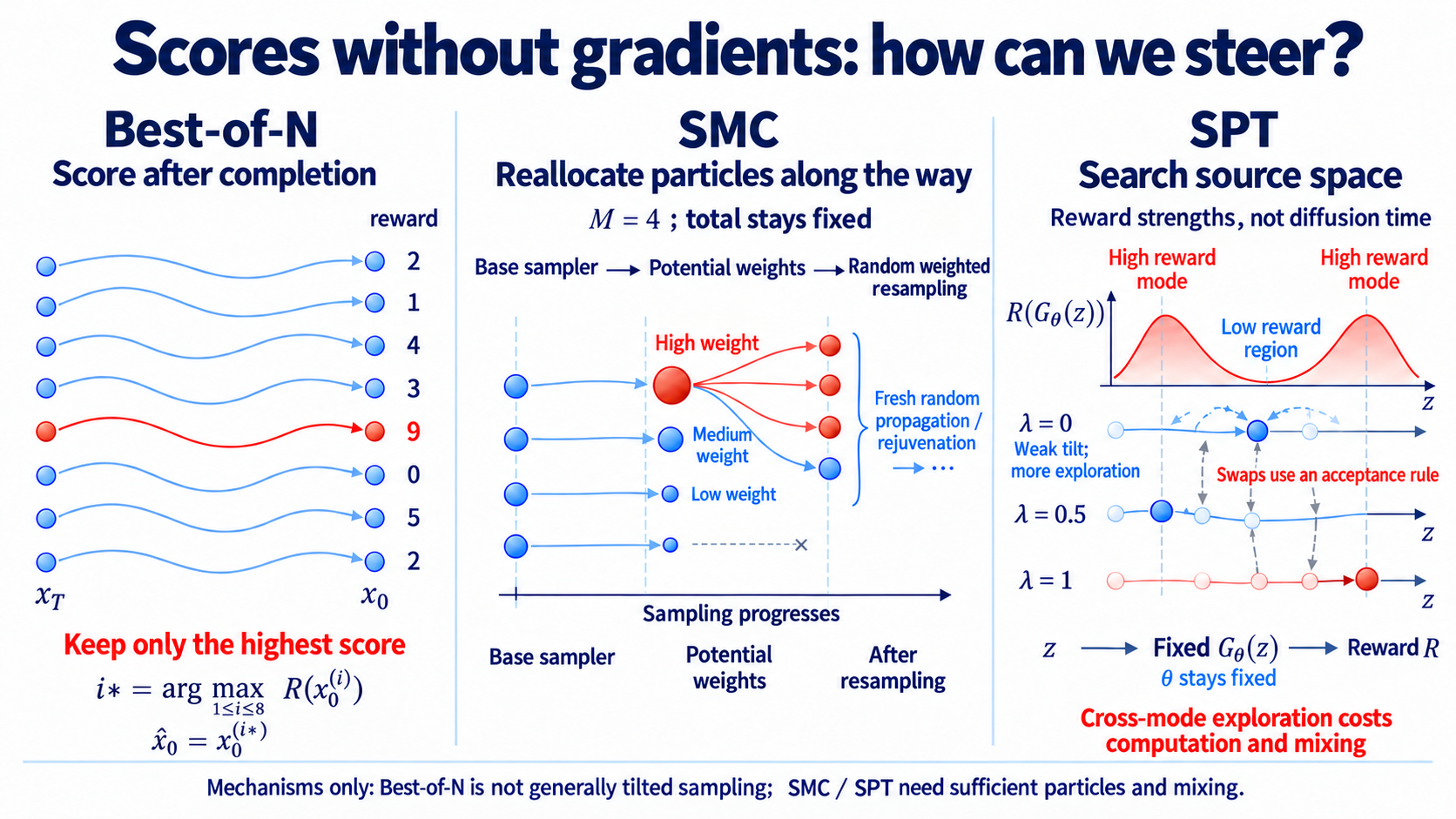
An evaluator that only gives scores can still steer: sample completed candidates by weight, resample drafts with incremental weights, or keep a deterministic generator and change source sampling. Finding a high-scoring image and approximating specified proportions require different checks. More computation does not automatically make them equivalent.
This overview connects terminal selection, intermediate resampling, and source search. SPT rows are reward strengths, not diffusion time. Its generator Gθ is our fixed G, while FK’s Gk−1 is a different incremental weight function. The mechanism drawing does not establish exact finite-computation sampling of pR.
Select the image to enlargeWhat if the model has not learned the data distribution exactly?
To examine sampling rules, we assumed a base of pdata. If the model actually outputs pθ, the same terminal weighting approximates the normalized distribution with weights
pθ(x0)eλR(x0).
With a finite-step sampler, the base is more precisely its actual output law, including discretization error. More candidates, particles, or chain exploration can improve approximation relative to that base, without automatically correcting it to pdata.
A result with no base support cannot appear through finite-reward reweighting. Even amplified low-probability regions may remain unseen by finite candidates. Model error, sampling approximation, reward, plausibility, and diversity therefore remain distinct checks.
Next, consider a more concrete request: the user supplies a blurry photo and wants a sharp image truly compatible with it. How should the evaluator score restoration of that photo, rather than simply a nice-looking dog?U7.4 continues from the measurement process.