L4.3 How can one kernel handle texture, objects, and an entire scene?

One kernel sees one scale

The previous note’s convolution looks at a small patch, while a photograph contains both detail and context. A map presents the same tradeoff: zoom out to see the route, zoom in to locate an intersection. Can a model preserve both kinds of information?

A photograph contains texture with periods of a few pixels, objects spanning tens of pixels, and composition across the whole image. Distinguishing cats from dogs might require both fur texture and ear shape, at very different scales.

A $K\times K$ kernel sees a region of side length $K$ . Start by stacking $d$ layers with stride 1 and no dilation. The receptive field describes the input region that can influence an output. Its side length is

\mathrm{RF}=1+d\,(K-1).

For $K=5$ :

  depth   1   RF =    5
  depth   2   RF =    9
  depth   4   RF =   17
  depth   8   RF =   33
  depth  16   RF =   65
  depth  32   RF =  129

The receptive field grows linearly with depth. Covering an offset of $128$ positions requires $32$ layers, each operating at the original resolution.

A $5\times5$ kernel needs $32$ layers to cover an offset of $128$ .
Halve the resolution every two layers, and $10$ layers cover $249$ positions.
Where did the discarded information go?

DiscussionQ1

Downsampling makes a large receptive field much cheaper. First calculate the saving, then ask: what information is discarded, and can we recover it?

Show the reasoning

First, the saving. After downsampling, the same kernel covers twice the distance in the original coordinates. Each layer adds $(K-1)$ times the current effective stride to its receptive field; every halving doubles that stride. With downsampling every two layers:

  depth   1   RF =    5   （stride 1）
  depth   2   RF =    9   （stride 2）
  depth   4   RF =   25   （stride 4）
  depth   6   RF =   57   （stride 8）
  depth   8   RF =  121   （stride 16）
  depth  10   RF =  249   （stride 32）

This table uses stride 2 in every second $5\times5$ convolution. In general, track

\begin{aligned} r_\ell&=r_{\ell-1}+(K_\ell-1)j_{\ell-1},\\ j_\ell&=s_\ell j_{\ell-1}. \end{aligned}

Here $r$ is receptive-field size and $j$ is the spacing between adjacent outputs in original-image coordinates. Smaller feature maps save computation at fixed channel count; increasing channels changes the total cost.

What is the price? Pooling combines adjacent values. A thin line, an exact boundary location, or a high-frequency texture may disappear when values are merged.

Upsampling alone cannot uniquely recover it. Replication or interpolation creates a higher-resolution signal from what remains. If distinct inputs produced the same pooled output, that output cannot tell us which input was present.

The decision is whether the task can afford this loss.

For a low-dimensional output, such as a class or score, some spatial detail may be irrelevant. Classification networks often progressively reduce resolution.
For an image-sized output requiring detail, such as segmentation, denoising, or generation, discarded boundaries may be exactly what the output needs.

A natural solution gives high-resolution features another route around the bottleneck. The encoder gathers broad context; the decoder restores resolution while receiving features from corresponding encoder levels. These are U-Net’s long skip connections. They are a common design, not the only possible architecture.

What exactly does downsampling destroy?

The phrase “high frequencies are lost” is qualitative. Let us measure it.

Take a cosine signal of length $64$ , apply $2\times$ average pooling, then restore its length with nearest-neighbor upsampling. Measure the remaining amplitude at the original frequency and the total reconstruction error.

    f   period (samples)   retained same-frequency amplitude   reconstruction error
    1        64.0                    0.9976                         0.0491
    2        32.0                    0.9904                         0.0980
    4        16.0                    0.9619                         0.1951
    8         8.0                    0.8536                         0.3827
   12         5.3                    0.6913                         0.5556
   16         4.0                    0.7071                         0.7071
   24         2.7                    0.1464                         0.9239
   31         2.1                    0.0024                         0.9988
   32         2.0                    0.0000                         1.0000

The final row is exactly zero. The period-two signal $+1,-1,+1,-1,\dots$ averages to zero in every pair. It is eliminated, not merely attenuated.

The table measures particular sinusoids under this particular filter and sampling procedure. It does not imply that every feature narrower than five or six pixels loses half its amplitude: signal shape, phase, and sampling matter too.

The rightmost column gives another perspective: a period-eight signal already has $38\%$ relative reconstruction error after one down-and-up cycle. Repeating the cycle processes an already altered signal.

Average pooling can map distinct inputs to the same output. Upsampling may guess missing detail, but it cannot turn discarded information into retained evidence.

This experiment does not establish a universal $s/5$ threshold. Check whether detail survives in channels, skips, or another representation. Reducing spatial resolution need not lose information: rearranging pixels into channels can be reversible.

CautionOne amplitude row is not monotone: sampling and aliasing matter

At $f=16$ (period $4$ ), the retained amplitude $0.7071$ exceeds the $0.6913$ at $f=12$ (period $5.3$ ). This is not simply measurement noise.

Downsampling makes some frequencies indistinguishable on the coarser grid: aliasing. Upsampling can also create spectral images. Distinguish Fourier amplitude from projection onto the original cosine, and account for phase and the special Nyquist case. A component at $f=20$ is higher-frequency than $f=12$ ; it should not be described as a newly created low frequency. These measurements do not define a universal attenuation cutoff.

The reconstruction-error column counts energy moved to other components as error too. In these two rows it increases from $0.5556$ to $0.7071$ .

Low-pass filtering before decimation reduces aliasing. Upsampling design also matters: unequal overlap and sampling artifacts can produce checkerboard patterns. Smoothing can help, but artifact mechanisms depend on the specific operators.

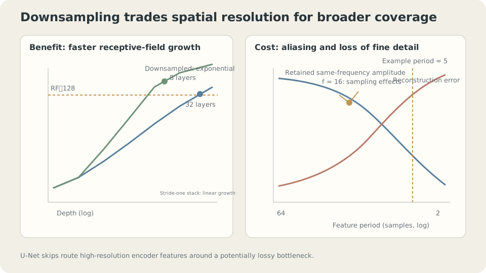
Receptive-field coverage and the information cost of downsampling

Figure: Downsampling expands coverage in original coordinates. Average pooling may lose detail, motivating a separate route for high-resolution information.

The line across the bottleneck

Q1 motivated the skip connection: information needed for a detailed output should have a route that avoids a lossy bottleneck.

Two connections are often called “skips,” but their main motivations differ:

U-Net’s long skip connects an encoder level to the corresponding decoder level, usually by concatenation. It carries high-resolution information around the bottleneck.
A residual connection, usually addition, writes $h_{l+1}=h_l+F(h_l)$ across a short block. It provides a direct signal and gradient route through a deep network.

These roles can overlap, but the distinction is useful: one preserves detailed features across scales; the other changes how depth is optimized.

The cost of depth itself

Depth introduces an optimization problem separate from receptive-field coverage. One Map, Different Starting Points: Loss Landscapes and Initialization examined gain; here we vary depth directly.

Use a $144\to32\to32\to\cdots\to1$ tanh stack with depths $8$ through $64$ . Compare plain layers, residual layers, and residual layers followed by LayerNorm. Train with Adam at $\eta=0.003$ for 1200 steps and report the median over three seeds.

First, output scale at initialization, for depth $32$ :

                 L1       L4       L8       L16      L32
  plain        0.2418   0.2265   0.1695   0.1513   0.0928
  residual     0.2418   0.5845   1.2501   2.5496   4.3765
  residual+LN  0.2418   1.0000   1.0000   1.0000   1.0000

The scales differ, but this table alone cannot identify every cause. LayerNorm [3] computes a mean $\mu(h)$ and variance $s^2(h)$ over designated feature dimensions:

\operatorname{LN}(h)=\gamma\odot\frac{h-\mu(h)}{\sqrt{s^2(h)+\varepsilon}}+\beta.

The normalized variance is exactly 1 only under idealizations such as ignoring $\varepsilon$ and omitting learned affine scaling. Practical LayerNorm outputs need not have variance exactly 1.

Next, compare gradient magnitudes: the ratio between the first and last hidden layers, with 1 meaning equal magnitudes.

  depth   4   plain 2.87e-01   residual 1.41e+01   residual+LN 2.71e-02
  depth   8   plain 7.05e-01   residual 5.61e+00   residual+LN 6.59e-02
  depth  16   plain 7.60e-02   residual 1.18e+00   residual+LN 1.74e-01
  depth  32   plain 6.47e-02   residual 7.64e-01   residual+LN 1.38e-01
  depth  64   plain 7.33e-02   residual 4.97e-01   residual+LN 1.29e-01

At depth $64$ , the residual ratio is closer to 1. Its local Jacobian contains $I+\partial F/\partial h_l$ , adding a direct branch. Other branches can still cancel or amplify gradients. This setting improves; residual networks are not universally immune to vanishing gradients.

Finally, training MSE:

  depth   8   plain 0.0000   residual 0.0000   residual+LayerNorm 0.0000
  depth  16   plain 0.0000   residual 0.0000   residual+LayerNorm 0.0000
  depth  32   plain 0.7399   residual 0.0000   residual+LayerNorm 0.0000
  depth  64   plain 0.9915   residual 0.0000   residual+LayerNorm 0.9096

Depth $32$ makes the motivation concrete. At the same width, data, and optimizer settings, the plain model stalls near a constant-prediction baseline, while the residual model fits to the displayed precision. The connection changes the parameterization and trainability, not just the nominal layer count.

Residual connections can make a deep model’s capacity easier to reach through training.

DetailsWhy is identity plus a small correction a useful starting point?

Write a layer as $h_{l+1}=h_l+F(h_l)$ . If the residual branch is initialized small, the block starts near identity. Many small changes can still accumulate, so a hundred such blocks need not jointly remain near identity.

This gives two useful possibilities.

First, a meaningful starting map. A small residual branch initially passes its input through, then learns corrections. The plain stack’s shrinking RMS suggests attenuation, although RMS alone does not prove that its output has lost all dependence on the input.

Second, an extra block can preserve a shallower map. If its residual branch can realize $F=0$ , the block is identity. This gives a simple way to embed a shallower computation in a deeper model, provided dimensions and other operations permit it. It does not guarantee that optimization finds that embedding.

The cost appears in the middle row: output scale grows from $0.24$ to $4.38$ as residual contributions accumulate. Architectures may scale residual branches, initialize a learned gate near zero, or use normalization. The appropriate scaling depends on depth and architecture; a fixed factor is not a universal remedy.

A deliberate counterexample: normalization is not free insurance

One number remains unexplained: at depth $64$ , residual training MSE is $0.0000$ , but residual plus LayerNorm gives $0.9096$ .

Normalization hurts this particular training setup. A familiar design choice still needs an experiment.

The gradient ratio provides a clue: $0.497$ for residual versus $0.129$ with LN. Normalization changes the gradient geometry, suppressing directions associated with uniform shifts and, approximately, positive scaling. But this ratio does not establish the unique cause of failure. Placement, affine parameters, and learning rate should also be compared.

LayerNorm nevertheless has a concrete scale property. Measure it:

  multiply W by   0.01 :  max|LN(XWc) - LN(XW)| = 6.853e-03
  multiply W by   1.00 :  max|LN(XWc) - LN(XW)| = 0.000e+00
  multiply W by 100.00 :  max|LN(XWc) - LN(XW)| = 6.874e-07

For positive rescaling and negligible $\varepsilon$ , the normalized output is approximately unchanged. The discrepancy at $c=0.01$ reflects the larger relative contribution of $\varepsilon=10^{-5}$ ; reducing it strengthens the invariance, subject to numerical precision.

The corresponding gradient scaling is:

  multiply W by  0.1 :  gradient norm for W = 178.238   (times c = 17.824)
  multiply W by  1.0 :  gradient norm for W =  17.824   (times c = 17.824)
  multiply W by 10.0 :  gradient norm for W =   1.782   (times c = 17.824)

For isolated $\operatorname{LN}(XW)$ , ignoring $\varepsilon$ and taking $c>0$ , the forward map is invariant to $W\mapsto cW$ , while its gradient scales as $1/c$ . The weight norm also grows by $c$ , so a fixed-step relative update scales as $1/c^2$ . It is not automatically constant. Biases, nonlinearities, and residual branches require checking the relationship again.

Normalization reduces sensitivity to feature scale while changing which gradient directions pass through. Whether this helps depends on the task and training setup.

Residual connections and normalization address related but distinct issues. Deep architectures often benefit from both, but this width- $32$ tanh experiment does not support adding this particular LN configuration automatically. It also does not establish that scale control is its only possible benefit.

In your own model, inspect per-layer output RMS, gradients, updates, and training curves together. Stable RMS alone does not show that normalization is unnecessary; compare its placement and hyperparameters directly.

Receptive field, frequency, and depth

Interactive demo: Downsampling, skips, depth, and connection type let you explore three separate questions: coverage, retained detail, and trainability.

Designing a U-shaped network

Turn the observations into a sequence of decisions.

Estimate the required receptive field. How far apart are the pieces of evidence the task must combine? Compare depth and downsampling to cover that distance.
Check which details must survive. Measure your actual filtering and sampling pipeline; there is no universal $s/5$ rule. When broad context and fine localization are both needed, compare a multiscale encoder with high-resolution skips.
Choose what the skip carries and how to merge it. Concatenation preserves separate channel representations at a higher channel cost. Addition is cheaper but requires compatible shapes and representations. Compare them for the output’s localization needs.
Inspect gradient routes. The toy’s depth thresholds are not universal. Examine gradients, updates, and training performance together.
Compare normalization configurations. Pre-norm, post-norm, affine parameters, and step size all matter. RMS alone cannot decide whether to use LN.

What do these decisions assume? Multiscale processing is useful when the data and task contain useful structure at several scales. Spatial downsampling needs a meaningful neighborhood structure. Finally, the depth and normalization results come from a narrow tanh stack; width, nonlinearity, initialization, and learning rate can change them. Repeat the measurements in your own setting.

Check your understanding

A task needs relationships between objects about $100$ pixels apart and boundaries only $3$ pixels wide. Which design direction is worth comparing?

Check your understanding

Which statement is incorrect?

References

Ronneberger, O., Fischer, P. & Brox, T. U-Net: Convolutional Networks for Biomedical Image Segmentation. MICCAI 2015.
He, K., Zhang, X., Ren, S. & Sun, J. Deep Residual Learning for Image Recognition. CVPR 2016.
Ba, J., Kiros, J. & Hinton, G. Layer Normalization. 2016.