U2.5 Lab: From Reference Paths to a Flow ODE

Fix the other experimental choices

Reuse the two-moons data, MLP, and random seed. Change the reference path, target, and sampler while controlling unrelated settings.

Our notation is

This is the opposite time direction to Unit 1.

Download the Flow Matching and ODE sampling notebook

Step 1: construct reference paths

Use linear Conditional Flow Matching [1]:

The training loop is

for step in range(n_steps):
    x0 = torch.randn(batch, 2)       # source
    x1 = sample_data(batch)          # target
    t = torch.rand(batch, 1)
    xt = (1 - t) * x0 + t * x1
    loss = ((model(xt, t) - (x1 - x0)) ** 2).mean()
    loss.backward(); opt.step(); opt.zero_grad()

The model receives position and time, with the reference velocity as its label. No density or explicit posterior weights are needed; regression performs the averaging.

A positive loss can remain because compatible reference labels disagree. The conditional-variance term is independent of the predictor. A nonzero CFM loss therefore does not by itself indicate a wrong marginal field.

Step 2: follow the learned velocity

Euler sampling uses

@torch.no_grad()
def euler_sample(model, x0, n_steps):
    x, h = x0, 1.0 / n_steps
    trajectory = [x]
    for i in range(n_steps):
        t = torch.full((x.shape[0], 1), i * h, device=x.device)
        x = x + h * model(x, t)
        trajectory.append(x)
    return torch.stack(trajectory)

Fix initial points and compare 10, 50, and 1000 steps. Check:

1. Does the endpoint distribution stabilize with resolution?
2. Do generated trajectories coincide with training reference lines?

Usually the second answer is no. Reference lines may cross, while trajectories of a regular unique ODE follow the average field without merging and separating.

Step 3: measure the cost of velocity changes

Use an exact field to remove neural estimation error and isolate numerical behavior.

On a log-log plot:

• Slope reflects convergence order in the asymptotic regime: approximately $-1$ for Euler and $-2$ for Heun under appropriate smoothness.
• Height reflects the error scale, including velocity variation and amplification along the trajectory.

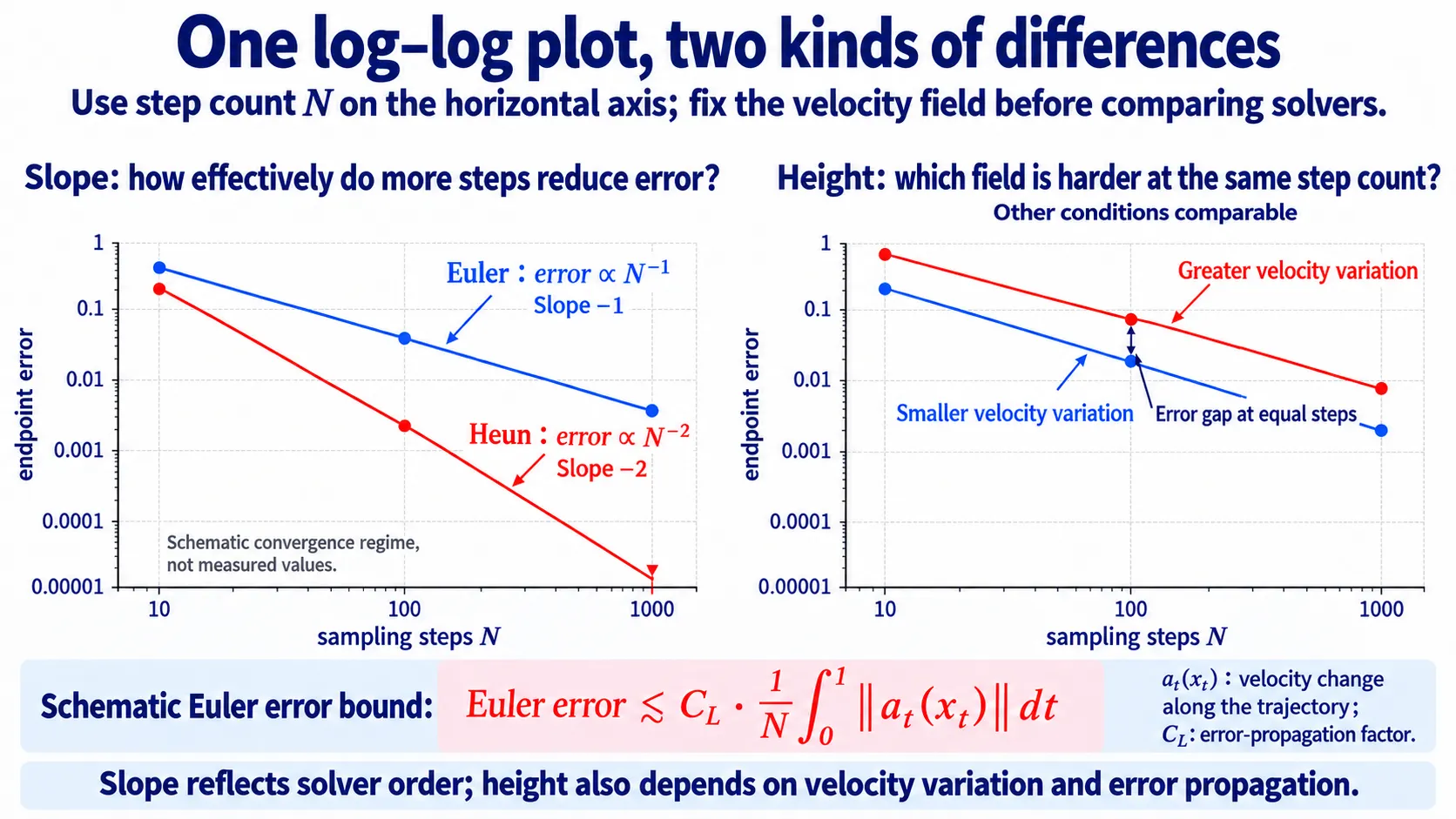
Figure: slope and height. The horizontal axis is step count $N$, with $h=1/N$. These are schematic curves, not measured results. U3.1 derives a more precise error bound.

Step 4: convert the diffusion denoiser to velocity

Load the VP-trained noise predictor and use the conversion from U2.3:

def eps_to_velocity(eps_model, x, t):
    a, s = vp_alpha(t), vp_sigma(t)
    da, ds = vp_alpha_dot(t), vp_sigma_dot(t)
    eps = eps_model(x, to_ddpm_time(t))
    return (da / a) * x + (ds - da * s / a) * eps

Integrate this field and compare with deterministic DDIM. As the grids are refined, the trajectories should approach the same continuous dynamics, assuming aligned time and coefficient conventions.

No. The coefficients in eps_to_velocity must match training. Output coordinates may change without retraining; an arbitrary intermediate distribution generally may not.

Exercises

1. Non-Gaussian source. Use a uniform source on $[-2,2]^2$, retrain, and identify which training and sampling code remains unchanged.
2. Coupling. Fix endpoint marginals and compare independent with position-based batch pairing. Plot reference paths, generated trajectories, and coarse-step errors.
3. Path. Fix pairing and compare linear with time-reversed VP interpolation. Measure marginal trajectories rather than inferring them from individual references.
4. Solver. Compare Euler and Heun on the same field and estimate convergence slopes. Also compare at equal network-evaluation budgets.

Check your understanding

References

1. Lipman, Y., et al. Flow Matching for Generative Modeling. ICLR 2023.
2. Karras, T., Aittala, M., Aila, T., Laine, S. Elucidating the Design Space of Diffusion-Based Generative Models. NeurIPS 2022.